Introduction
The use of AI in various industries has gained a lot of attention in the recent years. The textile industry is also starting to incorporate the technology in different parts of the product cycle. In this case, the students “Research Project Industry 4.0” are applying it at the end of the lifecycle of clothing. The goal is for the AI to be able to correctly identify and categorise different items of used clothing, automating the first part of the sorting process in a sorting facility for old clothing.
The AI in question has already been developed and trained in previous projects by the project partners “Striebel Textil” and the “Schülerforschungszentrum”. The students in this project worked to improve and further develop the artificial intelligence.
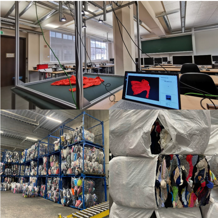
Figure 1: Research Project Industry 4.0; own presentation
Visit to the facility
Striebel Textil GmbH is a family-run company with over 30 years of experience in the recycling of used textiles. Every year, 7500 tonnes of used clothing are collected, sorted and sold (Striebel Textil , 2024).
In addition to the nationwide collection of used clothing from the containers of charitable partners, such as “Aktion Hoffnung”, and the sorting of used clothing, the company also collects, sorts and sells leftover stock from discounters. Used textiles that are no longer wearable and have the right material composition are also separated and sold to partners who process them into cleaning textiles and cleaning cloths.
Striebel Textil also operates its own second-hand shop. By working closely with charitable organisations such as “Aktion Hoffnung” and “Malteser”, the company makes a significant contribution to sustainability. The company combines social responsibility with ecological principles and thus plays a key role in the textile recycling sector.
(Striebel Textil, 2024)
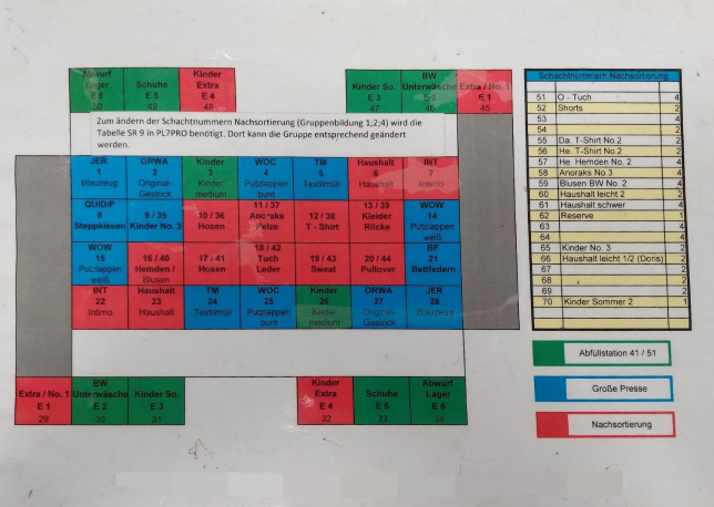
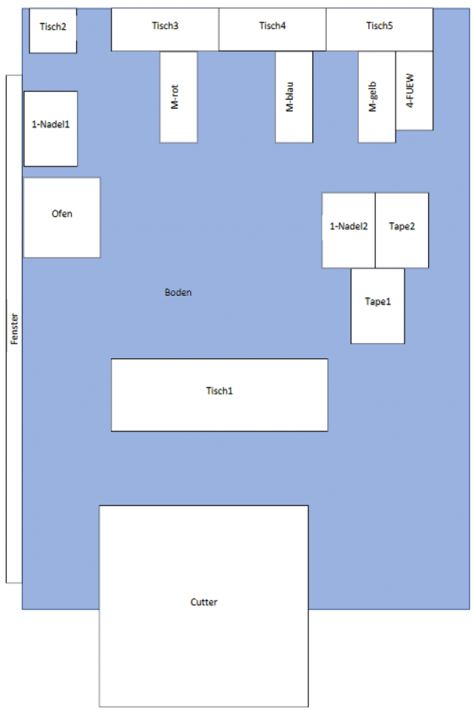
Figure 2: current categories of presorting; own presentation
Currently, the delivered goods first go to the pre-sorting area. There, the sacks are opened and sorted by thirteen employees into the categories listed in Figure 2 and then forwarded to the predetermined positions. As shown in Figure 2, some categories go directly to the large press, where the goods are pressed into bales and packaged. Other categories, such as individual shoes, are packed into bags in a filling station, while the categories marked in red are forwarded to the post-sorting area. At the post-sorting tables, the textiles are further sorted manually by employees according to category, condition, quality, brand and fashion.
The staff must be well trained in order to sort the used textiles as efficiently as possible according to the specified characteristics.
As the volume of used textiles has increased in recent years (Statistisches Bundesamt, 2024), Striebel Textil is working on solutions to speed up the sorting process. One approach here is to have the pre-sorting carried out by an AI. This would allow employees from pre-sorting to be deployed in post-sorting. It would also reduce the strain for these employees, as they would no longer be confronted with waste that is incorrectly placed in the containers or heavily soiled textiles.
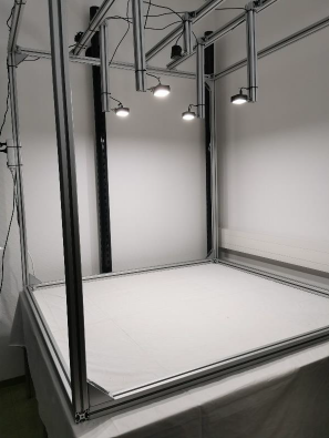
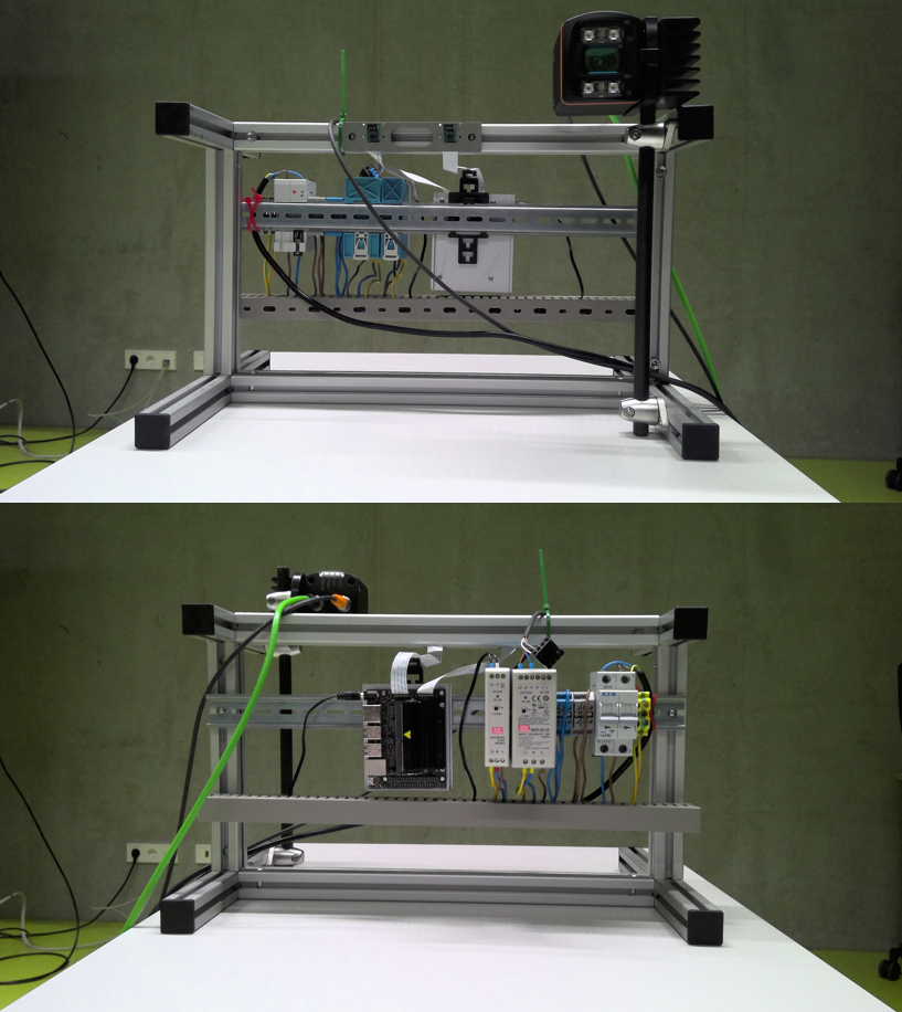
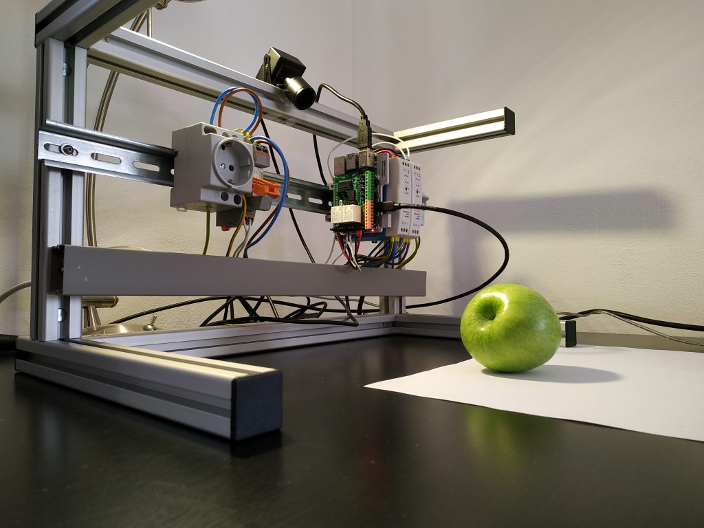
Figure 3: Photobox; own presentation
As mentioned at the beginning, the project started in 2023 with some students from the Kreisgymnasium Riedlingen, the student Benedikt Striebel from the Albstadt-Sigmaringen University of Applied Sciences and the Schülerforschungszentrum Südwürttemberg. The project was presented in the final of the national AI competition.
Here too, the aim of the project was to automate the first stage of sorting old clothes using AI. The team used an image recognition system based on AI to recognise individual items of clothing and assign them to specified categories. An existing neural network was used for this, which was trained with corresponding image data.
A photo box was constructed to create the image data in order to ensure consistent lighting conditions and a consistent image section Figure 3. A white cloth was used as background. To ensure more even lighting, four Rollei LUMIS Mini LEDs were used and the images were created using a Logitech StreamCam, which allowed the images to be created and processed in Full HD quality directly via a computer. The images created then had to be categorised.
In this previous project, around 2000 images were created from unsorted goods and assigned to the corresponding categories. (sfz, 2024)
As part of the project, the entire training process was to be improved. This also involved making further adjustments to the photobox. As there were frequent problems with recognising white textiles on the white background in the previous project and the pre-sorting will later take place on a conveyor belt, a dark green fabric background was chosen as this has a similar colour to the future conveyor belt. In addition, the image section was adapted to the dimensions of the conveyor belt that would later be used (256x384px). To improve the image quality and therefore object recognition, the old webcam was replaced by the industrial webcam “IDS u-eye u36-l0xc”. It has an automatic focus and an automatic white balance, which means that both light and dark colours are easily recognisable on the background.
Preparation
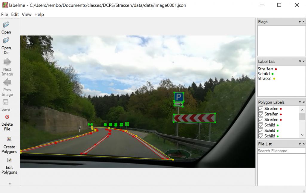
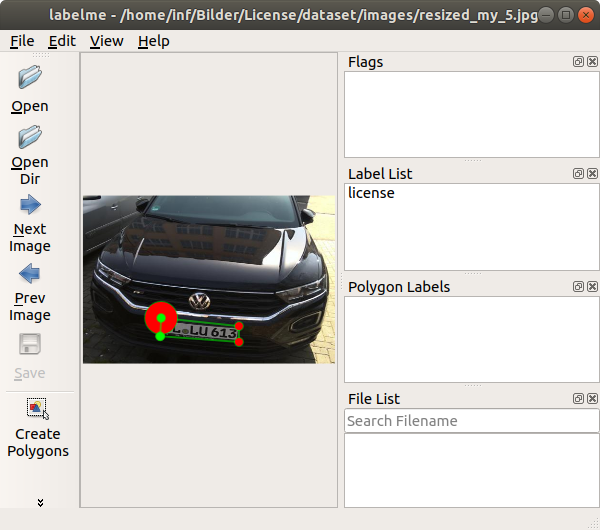
Defining new categories
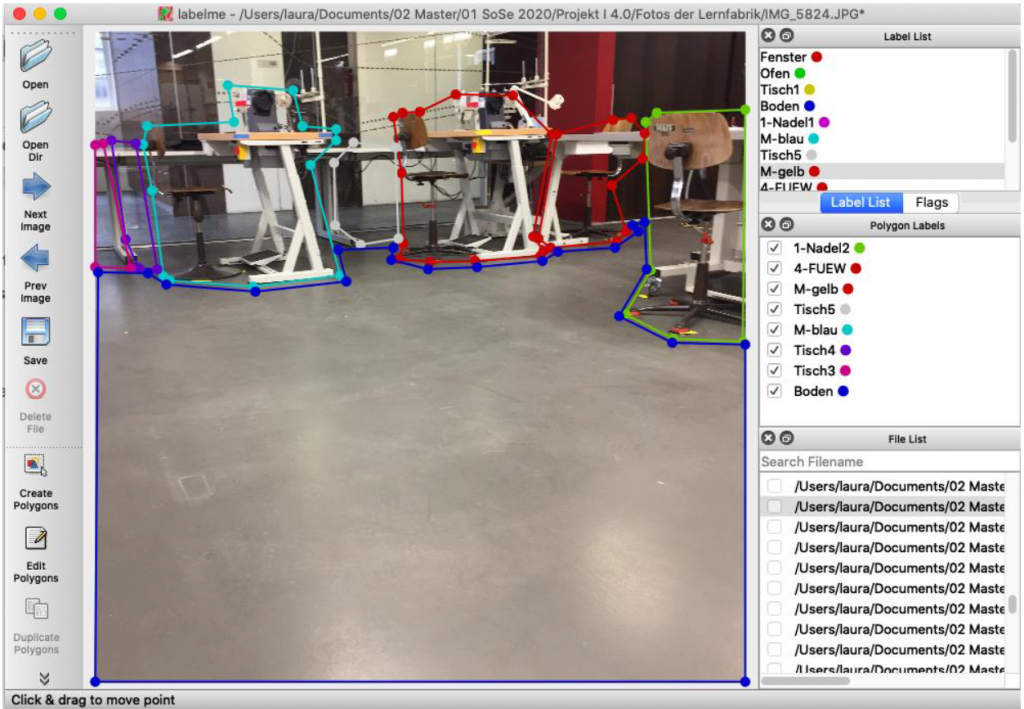
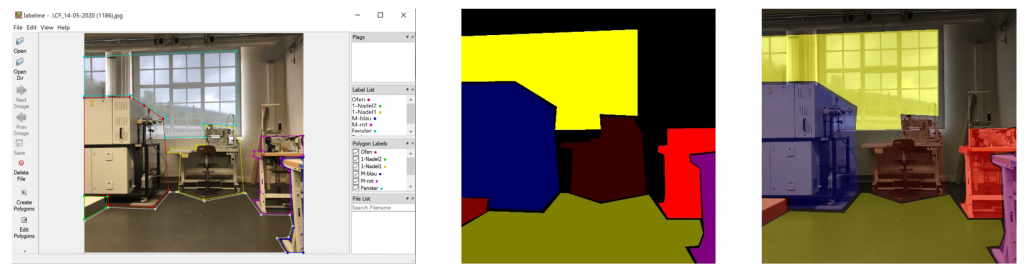
One of the most important parameters for the recognition of textiles with AI is the labeling process. To be able to train the AI afterwards, defined labels are necessary. Therefore, as part of the project, the images are labeled with the textile categories. By selecting the corresponding category, the current live image from the camera is saved and stored in the respective category folder so that the AI can be trained next.
The previous labeling process was carried out on unsorted garments. Therefore, the selection of categories was based on the garments available in the used clothing bags without considering the categories used in the company. As a result, some categories were not included in the training. In addition, not every category had the same number of pictures, which later led to overtraining of categories.
The previously used categories amounted to the following 13 categories:
- Gloves
- Pants
- Jackets
- Children’s clothing
- Dresses
- Hats
- Sweaters
- Scarves
- Shoes
- Socks
- Bags
- T-shirts
- Underwear
The project focused on defining and labeling new categories. The basis was the sorting system already established in the company (Figure 2). This system was adapted and implemented in the program.
The following 26 categories were selected in advance and adapted during the process:
- Children’s clothing: Underwear
- Blankets
- Children’s clothing: Shirts / blouses
- Plush toys
- Children’s clothing: Pants
- Shirts / blouses
- Children’s clothing: sweatshirts & T-shirts
- Sweaters / original knitwear
- Children’s clothing: sweaters
- Pants
- Children’s clothing: jackets
- Cloth / leather
- Children’s clothing: dresses & skirts
- Anorak & furs
- Cotton underwear
- T-shirts & sweatshirts
- Intimo underwear
- Dresses & skirts
- Socks
- Textile waste
- Shoes
- Garbage
- Towels
- Cushions
- Bath rugs
- Comforters
Previously one of the biggest challenges was to ensure that children’s clothing was correctly identified, as the AI tended to label clothing that was not clearly identifiable as children’s clothing, as this included all items of clothing such as pants, dresses and skirts. The approach to minimize these misclassifications was to divide the children’s clothing into sub-categories to simplify the identification of the garments. The categories defined for children’s clothing were based on the categories already defined for adult clothing.
Final category system
However, the previously defined categories had to be adapted as the project progressed. The underwear category was not differentiated between cotton and intimate apparel as intended, as there was too little image data available for these categories. It was decided that the subdivision would take place later in the post-sorting process.
In the course of the project, it was decided to divide the sweatshirts & t-shirts category into two categories, “long-sleeved” and “short-sleeved”.
In addition, the category of shoes was subdivided into single pairs and paired shoes, because if the shoes are only available as separate items, they are sorted out and sold to a third party.
The household category was defined for blankets, bedding and carpets, as the classification turned out to be more difficult during the process. In the sorting system already being used, these categories are under the household category, so no further separation is considered necessary.
Unlike previously intended, the AI is not actually trained with items of waste for a separate category, but instead the items are assigned to this category based on a particular percentage score. The exact percentage has not yet been determined at this stage, as it is still necessary to test at which point the AI can no longer recognize the textile accurately. Therefore, items that the AI cannot clearly recognize will be assigned to the category “waste”.
During the training process, the previously defined categories were revised again and adapted for the training process. The final categories of the labeling process are listed below.
- Anoraks furs
- Comforters
- Blankets
- Towels
- Shirts-Blouses
- Pants
- Children’s pants
- Children’s jackets
- Children’s dress-skirts
- Children’s short sleeves
- Children’s long sleeves
- Children’s underwear
- Pillows
- Dress-skirts
- Garbage
- Plush toys
- Sweater knitwear
- Shoes
- Pairs of shoes
- Carpets
- Textile waste
- T-shirts-Sweatshirts
- Cloth-Leather
- Undefined
- Underwear
Training
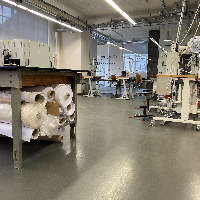
In order to start creating images for the Training Data, the previously built photo box first had to be transported to the university facility. The other option was to carry out the training data on site at Striebel Textil GmbH, but this would have taken more time. However, the already pre-sorted used textiles had to be brought to the university facility.
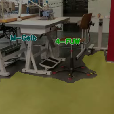
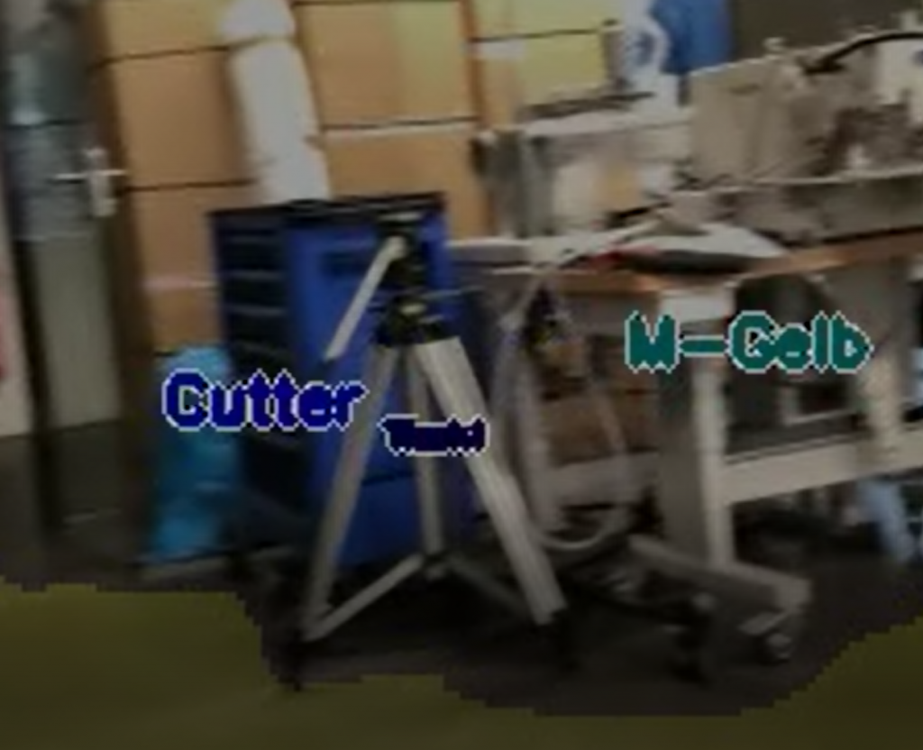
Once everything was in place, we could start the training process. To ensure consistent conditions in the process we would cover the windows and turn on the lights in the room we worked in. We turned on the LED-lights next to the camera and made sure we wouldn’t step too close to the box while taking pictures to avoid creating shadows.
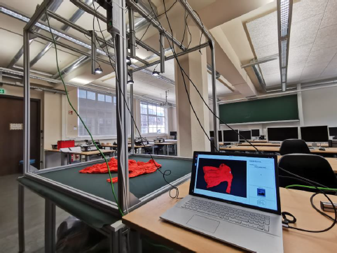
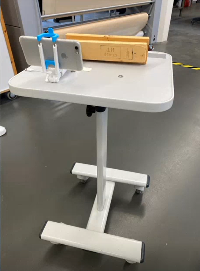
Figure 4: Set up for image taking (window in back not yet covered) covered); own
presentation
The process of the previous image-process was as follows: A bag of unsorted old clothing was opened, and individual items were taken out. Then they would be categorized, which sometimes involved long discussions, because different items could sometimes fit into more than one item group or would be otherwise harder to classify. Afterwards the item could be placed into the box and a photo would be taken and put into the respective category. The number of items that were categorized was determined by the number of items of this group that was present in the chosen bags.
Based on what we learned about the pervious results of the project we knew we needed to make some improvements to the image-making process. We had to decide how many images we would take in each of the newly defined categories. By setting a certain number of images that we would aim for, we would ensure that all categories would be equally well trained. This would hopefully help stop the AI’s tendency to put items it was unsure about into over-trained categories while also struggling with the under-trained ones.
We decided to aim for roughly 300-360 images in each category. The following table shows our total amount of images taken and the number of images in each category:
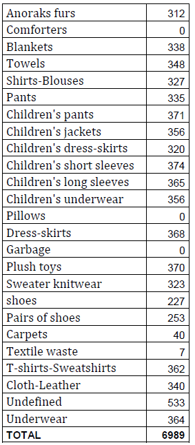
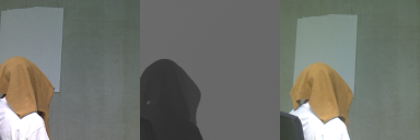
It is noteworthy that no pictures were taken in three of these categories. The reason for this was that the comforters and pillows were to be sorted with the help of 3D camera depth information so that these categories can be distinguished from the blankets category. As previously stated, we didn’t take any images for the garbage-category, intending items to be sorted into that category if they fail to reach a certain percentage in other categories. The textile-waste-category was also not trained properly, since the textile waste will later be sorted together with the other waste.
The category “undefined” included images form different categories, which have not yet been sorted. These included items form the household category and items we were unsure of.
To speed up the process and make sure we would have enough products to take the images with, we picked up multiple bags of pre-sorted clothing articles from Striebel Textil GmbH. By doing this we could be more certain about which items belong into which item group. Having a whole bag of t-shirts for example also means that we can put one item after the other into the photo box without having to discuss which product group it belongs into and without constantly searching and changing the category in the program. This didn’t mean we never had to debate which item belongs into which item-group.
Sometimes the pre-sorted bags contained items that were incorrectly thrown into the product-group. These were then discussed if necessary and put into the correct category.
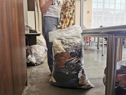
Figure 5: Taking a dress out of the bag full of presorted dresses and skirts ; own
presentation
Other times we noticed that there were problems with our new categories. Certain item-groups were not considered before and then came up during the image-making process. Some groups had to be reconsidered and renamed like for example the “household” category, which was first separated into “bedding”, “bath rugs” and “towels”. During the process we also noticed a big number of pillowcases and curtains, which also needed to be sorted, but didn’t have a separate group. Because of that and due to the visual similarities between pillowcases, blankets, carpets and similar items, we decided to group these items together. Other categories, like the “textile waste” and “trash” categories, have been deleted again.
Once it was clear which group the item belonged to, we would put it into the photo box and wait for the camera to focus so we could take an image of it which is saved with the program “texLabeler”, which was designed by our project partner. Usually, we would make multiple images of one item. Those images would show the item in different positions on the backdrop, including front and back view. By doing so, we could fill up the categories without having to transport hundreds of items to and from the university. Since the AI will be used in a less controlled environment the clothing pieces will not always lay perfectly flat. This is why we made sure to crumple up the items and twist them into different positions. Sleeves and pant legs would be folded over or beneath. This was supposed to help train the AI to work under less perfect and controlled conditions.
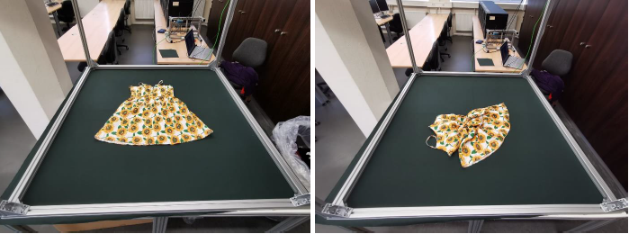
Figure 6: One dress in two different positions, one laying flat and one crumbl ed up
The photographed items were put back into their bags and returned to Striebel. Once all the categories were finished the AI could be trained.
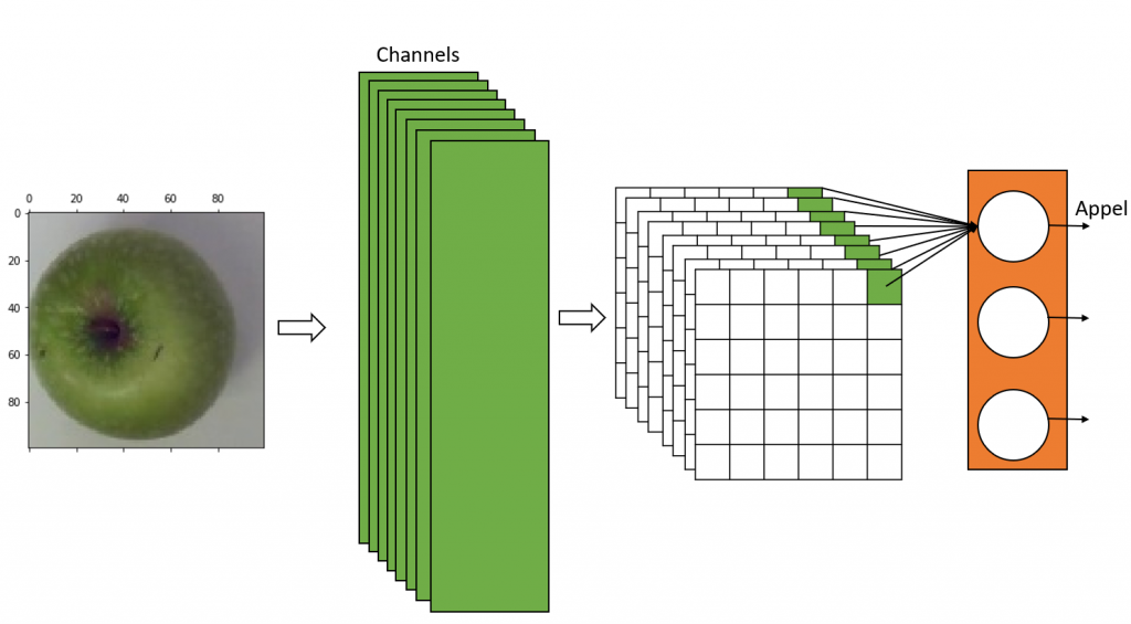
Since the goal of this project was to improve an already existing and tested AI, the focus was put onto the textile side of things. In addition to that we only had limited contact with the programming side of things, since this was taken over by our project partner. Because of that we will only provide a brief explanation as to how the AI works in order to create a general understanding of the topic.
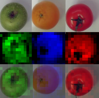
The images we’ve taken are forwarded to the training. The AI model is trained with all the images in the training dataset, passing them through the model with their assigned labels. Some images go through the Torchvisions transform module, which applies trans-formations like rotating, slightly shifting, flipping and recolouring to the images, artificially generating “new” images, which are also added to the training.
The training is either carried out for a certain number of epochs or in an endless loop. An epoch refers to one complete pass through the entire training dataset. During the training the AI tries to identify typical patterns for each category, building its own model.
After the training the model is validated. This is done with images from the validation dataset. These are images, which have not been trained before and which are unknown to the AI. The AI can then test itself, by guessing the categories of the validation images and checking its answer with the provided labels.
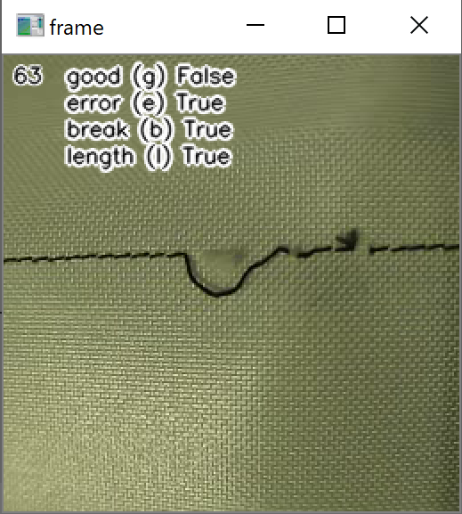
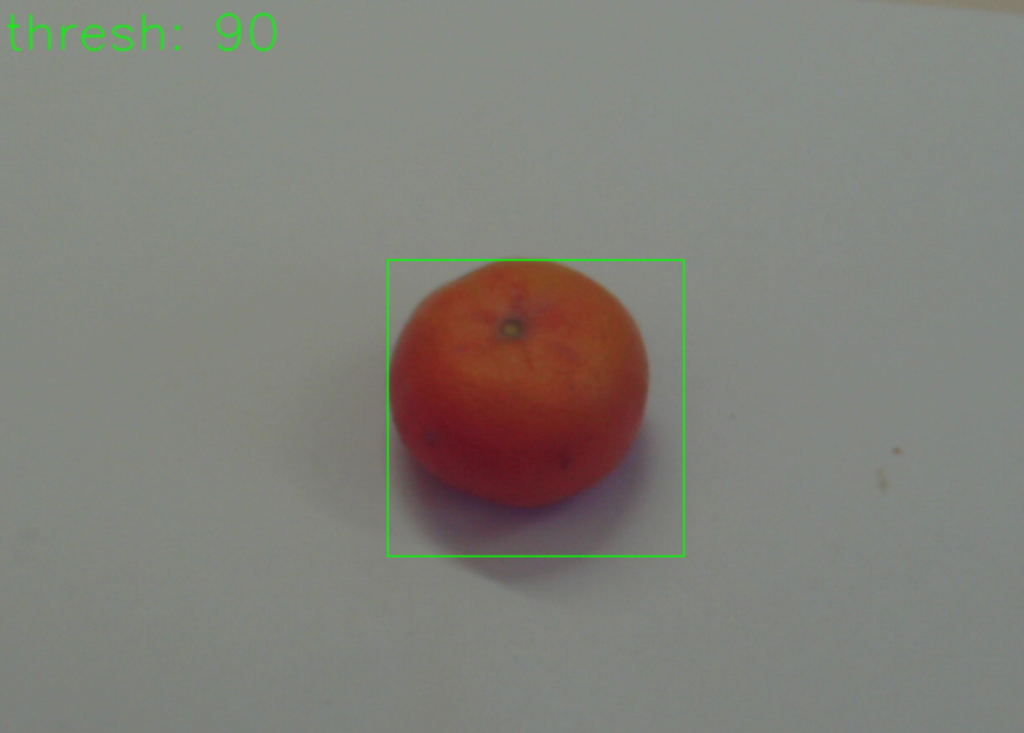
With the help of “texIdentifier”(Figure 7), another program created by our partner, we could test the trained AI with image files or directly via a camera. The program then shows how likely the object in the image fits into the different categories. The category with the highest probability is the one in which the AI would categorise the object and is prominently shown above all other categories.
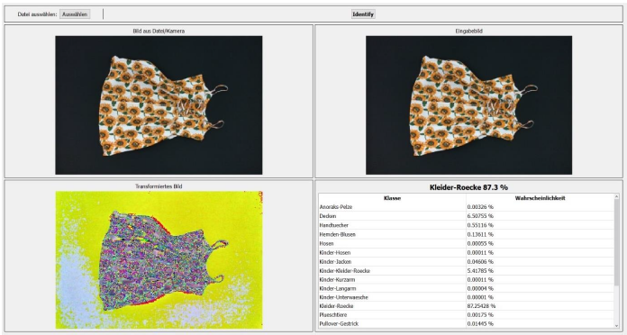
Figure 7: texIdentifier
The last program “texPlotter” shows the losses and accuracies of the training in a diagram and displays how the AI evolved over the training period.
After our first training session with the learning architecture ResNet50 we noticed an overfitting problem. This meant that the AI was too focused on the training data, which rendered it unable to work with new images which were not part of the training dataset. This can be seen in Figure 8. The blue line showing the training is smooth and shows good results, while the orange line showing the validation data is showing very notable spikes.
This led to incorrect results when testing the trained model. Many of the items were put into the wrong category. Dresses and T-Shirts were often identified as blankets or towels for example. It turned out to be due to a mistake in the test program in which the images were not set to the correct size.
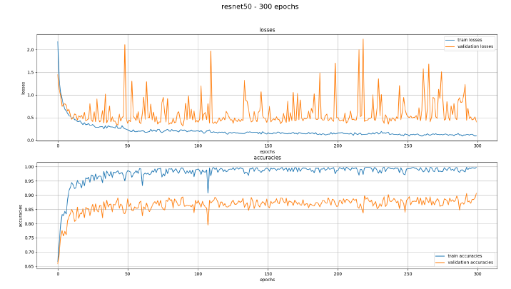
Figure 8: texPlotter with overfitting problems
After correcting the mistake, the following training produced much more promising results. The system still isn’t perfect though. While testing we noticed that pants with bold patterns and prints are more likely to be mistaken for dresses, even if the pantlegs were clearly visible. Items like towels and blankets are sometimes getting mixed up due to their shape, but they will be sorted together in the blanket category “household” anyway.
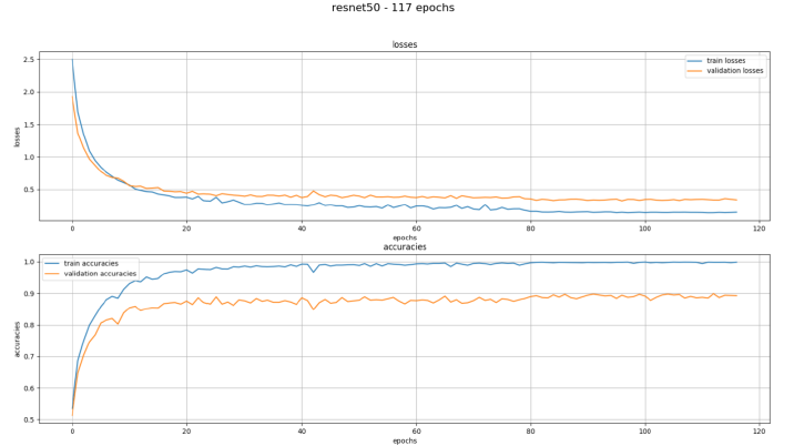
Figure 9: texPlotter after correcting the mistake
The graph shows the losses and accuracies with the pretrained model resnet50 trained with 117 epochs. The blue line shows the training and the orange one the validation. It can be seen that there is a quick drop at the beginning, which is expected and desired. In the course of the training the lines of the losses run towards zero, which means the AI is making fewer and fewer mistakes in both the training and the validation data.
In the accuracies both lines increase towards 1.0 accuracy, but the validation accuracies stop at 0.9. This means that the AI is not achieving 100% accuracy but only 90% with the validation data, which is also to be expected and is a good result.
The training did not proceed over the 117 epochs in this case, to avoid overfitting the model once again.
Improvements
, further ideas and next steps
During the process, the categorisation criteria required further adjustment. In order to continuously optimise the AI and comprehensively incorporate all categories, additional modifications to the categorisation schema will be necessary. Beyond establishing categories and training the AI, it is essential to consider methods for separating the textiles into individual items so that the AI can accurately identify them later. Various approaches to achieve individualisation have already been explored by others, for example in industrial settings, vibrating tables are commonly used for the individualisation of goods. The vibration helps separate products from one another. However, the properties of textiles present significant challenges in this context. Textiles have a low modulus of elasticity and low tensile rigidity, meaning that even minimal force can cause significant deformation. Robots capable of handling pliant materials have already been developed. A further solution could be the use of a Tesla Bot to assist in placing textiles individually on the conveyor belt, although this is not a viable solution in the near future.
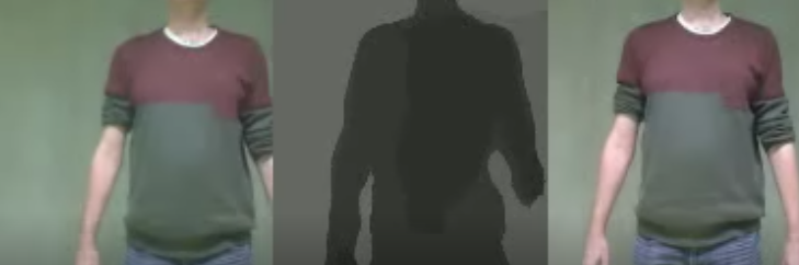
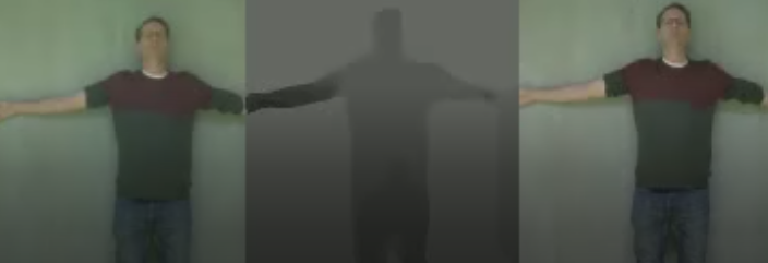
As previously stated, the incorporation of a 3D camera into the labeling process is a potential avenue for consideration. The advantage of utilizing a 3D camera is that it provides depth information in addition to two-dimensional values. This feature would be particularly beneficial for distinguishing between categories such as pillows and duvets from their respective covers. Similarly, depth information would assist in differentiating between socks and shoes. Initially, the integration of a scale into the conveyor belt was considered to provide the AI with weight data in addition to visual information, as these categories can be effectively distinguished based on weight. This idea was put aside, since the use of a 3D camera could be used for the differentiation while also being easier to integrate into the process.
During the project, an excursion to the facility was conducted. It was noted that individual shoes are directly sorted out in the pre-sorting process and sold to a third party. This presents a significant opportunity to enhance the AI in the future to identify matching pairs of shoes, by storing and analysing the captured images to identify pairs based on their data.
In the post-sorting process, products are not only sorted according to quality, but also in accordance with current trends. To later on incorporate AI into post-sorting, the AI could be trained to recognise and consider current trends in the textile industry. This approach would enable the AI to assist in sorting based on both quality and market trends, thereby further improving the efficiency and relevance of the sorting process.
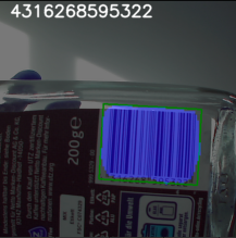
The issue of textile waste is becoming increasingly pressing, necessitating the development of innovative solutions to enhance the efficiency of recycling operations. Some measures can be taken even prior to the sorting process of old textiles. The integration of Radio-Frequency Identification (RFID) chips into textiles during the production process represents a promising approach to improving the sorting and recycling of old textiles.
RFID technology involves the embedding of small chips that can store and transmit data when scanned by RFID readers. These chips can be sewn into garments and other textile products without affecting their use or appearance. The data stored on these RFID chips includes detailed information about the textile’s material composition, manufacturing process, and dye types. This information is crucial for the effective recycling process. Upon scanning a textile item with an RFID chip, the recycling system is able to instantly determine its composition. This level of accuracy reduces contamination of recyclable materials and improves the quality of the output.
However, to facilitate the widespread adoption of RFID technology in textiles, legislative changes are necessary to mandate the integration of these chips during production. It is imperative that governments provide active support for these initiatives, implementing policies and incentives that encourage manufacturers to adopt sustainable practices and significantly reduce textile waste.
It is also to be noted, that we are not the only ones working on this topic, A similar project has been carried out by the Augsburg Institute for Textile Technology and the Institute for agile Software Development. Their project also aimed to train an AI to automatically identify and classify old clothes. For this they used a similar set-up, adding one camera for close-up images of the textiles. Instead of relying only on the images of real clothing items, they integrated artificial images with the help of generative models like StableDiffusion. By doing so they could reach a higher count of training images in a short time. This project is showing promising results but, according to the creators, still has a need for improvement in the areas of classification and the detection of interfering materials. (Sebastian Geldhäuser, 2024)
Results / Conclusion
In conclusion, our project shows promising results. The categories have now been systematically improved and can be used in the further development of the AI. There will certainly be more adjustments to them, but this is a good place to start. Our changes in camera and background have successfully contributed to the improvement of the AI and the new training results are promising. We have also already discussed and pointed out further ideas and areas of improvement. Although we made steps in the right direction, there is still a lot to be improved and considered, before the AI can finally be incorporated in the pre-sorting process to help improve textile recycling.
Acknowledgements
We would like to thank the Schülerforschungszentrum for the continuous support of this project. Additionally, we would like to thank Mr. Lehn for his support and help with transporting the photobox and the sacks for the project. And finally, we would also like to thank Benedikt Striebel for the great and straightforward collaboration and the many hours of work he invested in the project.
Sources
- Sebastian Geldhäuser, M. C. (2024). Die Zukunft der automatisierten Sortierung von Alttextilien. Melliand Textilberichte 3.
- sfz. (17. 06 2024). Von https://sfz-bw.de/2023/11/projekt-ai-recyclotron-im-finale-des-bundeswettbewerbes-ki/ abgerufen
- Statistisches Bundesamt. (17. 06 2024). Von https://www-genesis.destatis.de/genesis//online?operation=table&code=32121-0001&bypass=true&levelindex=0&levelid=1718625028992#abreadcrumb abgerufen
- Striebel Textil . (17. 06 2024). Von http://f2594702.td-fn.net/index.php?Sortierung abgerufen
- Striebel Textil. (17. 06 2024). Von https://www.striebel-textil.de/ abgerufen