Fruit Recognition on a Raspberry Pi

As a instructor I offer a class, in which I let master students choose a topic for practical work during a semester. I usually give them a rough description, which included last time a raspberry pi, a camera, and a neural network.

Some students have chosen to work on fruit recognition with a camera. So the scenario is the following: The camera is connected to a raspberry pi. The camera observes a clean table. As soon as a user puts a fruit onto the table, the user can hit a button on a shield attached on the raspberry pi. The button triggers the camera to take an image. Then, the image is fed into a trained neural network for image categorization. The category was then fed into a speech synthesizer to speak out the category.

The type of neural network my students and I used is a multi-categorical neuronal network. So the goal was to feed the neuronal network with image and a category will come out as an output.

Preparing the Data

In the beginning we chose fruit images from a database which is available on github. You find it here. It had about 120 different categories of fruits and vegetables available. The problem we find with these images are, that the fruits and vegetables seemed to be perfect looking which is in reality not the case. The variation of fruit images within one category also seemed to be very limited. On the one hand, they do have many images within each category, on the other hand it looks like each image from one category only comes from a perfect fruit photographed in different positions.

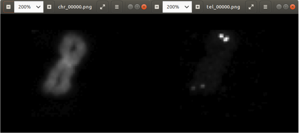
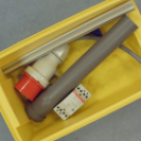
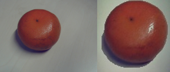
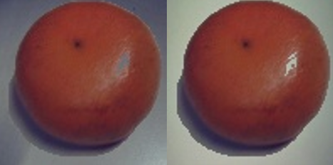
The fruits fill out the complete image, as well. When you photograph a fruit from a table, this is in general not the case. The left part of Figure 1 shows an orange which fills in only part of the image.

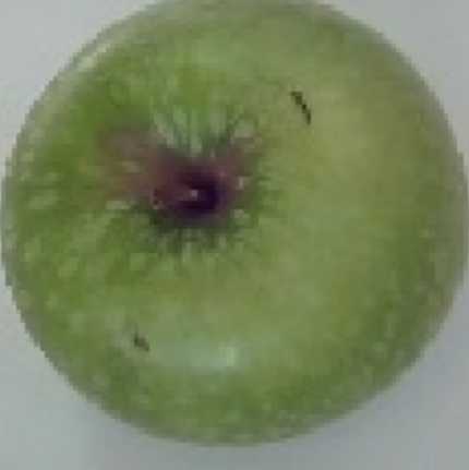
What is more, the background of the images from the database is extremely bright. This is not quite a real life background, which we find is much darker when you take pictures from inside a building. In Figure 2 you can see two different backgrounds which are surfaces from two different tables. The backgrounds do have relatively low brightness.

Cropping the images

The first task was to prepare the data for training the neural network. We decided to crop the images to the size of the fruits, so we receive some kind of standardization of the images. Below you find the code which crops the images to the size of the fruit. In this case we have the fruit images inside the addfolder. Inside the addfolder we first have two more directories, Testing and Training. Below these directories you find the directories for each fruit. We limit the number of fruits to six. The fruits we use are listed in dirlist, which are also the directory names.

The code is iterating through the Testing and Training directories and the fruit directories in dirlist and loads in every image with the opencv function imread. It converts the loaded image to a grayscale image and filters it with the opencv threshold function. After this we apply the findContours function which returns a list of contours of the image. The second largest contour (the largest contour has the size of the image itself) is taken and the width and height information of the contour is retrieved. The second largest contour is the fruit portion on the image. The application copies a square at the position of the second largest contour from the original image, resizes it to 100×100 pixels and saves it into a new directory destfolder.

srcfolder = '/home/inf/Bilder/Scale/orig/'
destfolder = '/home/inf/Bilder/Scale/cropped/'
addfolder = '/home/inf/Bilder/Scale/added/'
processedfolder = '/home/inf/Bilder/Scale/processed/'

dirtraintest = ['Testing', 'Training']
dirlist = ['Apfel','Gurke','Kartoffel','Orange','Tomate','Zwiebel']

count = 0
pattern = "*.jpg"
img_size = (100,100)

for traintest in dirtraintest:
    for fruit in dirlist:
        count = 0
        for file in glob.glob(os.path.join(addfolder, traintest, fruit, pattern)):
            im = cv2.imread(file)
            imgray = cv2.cvtColor(im, cv2.COLOR_BGR2GRAY)
            ret, thresh = cv2.threshold(imgray, 127, 200, 0)
            contours, hierarchy = cv2.findContours(thresh, cv2.RETR_TREE, cv2.CHAIN_APPROX_SIMPLE)
            if len(contours) > 1:
                cnt = sorted(contours, key=cv2.contourArea)
                x, y, w, h = cv2.boundingRect(cnt[-2])
                w = max((h, w))
                h = w
                crop_img = im[y:y+h, x:x+w]
            im = cv2.resize(crop_img, img_size)
            cv2.imwrite(os.path.join(destfolder, traintest, fruit, str("cropped_img_"+str(count)+".jpg")), im)
            count += 1

Figure 1 shows how the application crops an image of an orange. On the left side, the orange fills out only part of the image. On the right side, the orange fills out the complete image.

Figure 1: Original Image and Cropped Image

Changing the backgrounds

Due to the extreme bright background of the images from the database we came to the decision to fill in new backgrounds on top of the bright ones. In Figure 2, you can see two different table surfaces, taken by the camera we used.

Figure 2: Backgrounds

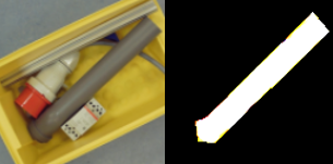
The code below shows how each image from the directory structure (which I explained above) is loaded into the variable pixels with the opencv imread function. Each pixel on each layer (RGB) of the image is checked, if a threshold of brightness has been reached. We assume that a pixel exceeding a certain brightness threshold is a background pixel (which is not always the case). The application then replaces the pixel with a pixel from a background image shown in Figure 2. It saves the new image to the directory processedfolder.

background = cv2.imread("background.jpg")

bg = np.zeros((img_size[0], img_size[1],3), np.uint8)
bgData = np.zeros((img_size[0], img_size[1],3), np.uint8)

bg = cv2.resize(background, img_size)
bgData = bg.copy()

threshold = (100, 100, 100)

for traintest in dirtraintest:
    for fruit in dirlist:
        count = 0
        for name in glob.glob(os.path.join(destfolder, traintest, fruit, pattern)):
            pixels = cv2.imread(os.path.join(destfolder, traintest, fruit, name))
            pixelsData = pixels.copy()

            for i in range(pixels.shape[0]): # for every pixel:
                for j in range(pixels.shape[1]):
                    if pixelsData[i, j][0] >= threshold[0] and pixelsData[i, j][1] >= threshold[1] and pixelsData[i, j][2] >= threshold[2]:
                        pixelsData[i, j] = bgData[i, j]
            cv2.imwrite(os.path.join(processedfolder, traintest, fruit, str("processed_img_"+str(count)+".jpg")), pixelsData)
            count += 1

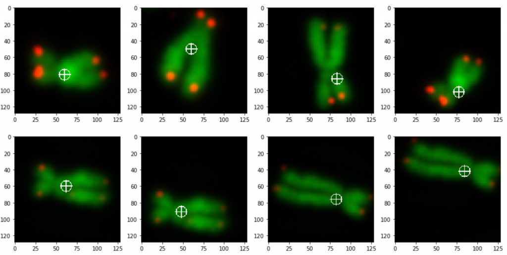
Figure 3 shows the output of two images from the code above. It shows the same orange with two different backgrounds.

Figure 3: Orange with two different Backgrounds

Training the Model

Below the code of a neural network model. It consists of four convolutional layers. The number of filters is increased with each layer. After each convolutional layer there is a max pooling layer to reduce the image size for the input of the following layer. A flatten layer follows and is fed into a dense layer. Finally there is another dense layer with six neurons. This is the number of categories we have. Each layer uses the relu activation function. In the last layer however we use the softmax activation function. The reason for softmax, and not sigmoid, is, that we expect only one category from the six categories to be true for a given input image. This can be represented by the highest number calculated from the six output neurons. For optimization, we use stochastic gradient descent method.

model = Sequential()
model.add(Conv2D(16, (3, 3), activation='relu', kernel_initializer='he_uniform', padding='same', input_shape=input_shape))
model.add(MaxPooling2D((2, 2)))
model.add(Conv2D(32, (3, 3), activation='relu', kernel_initializer='he_uniform', padding='same'))
model.add(MaxPooling2D((2, 2)))
model.add(Dropout(0.1))
model.add(Conv2D(64, (3, 3), activation='relu', kernel_initializer='he_uniform', padding='same'))
model.add(MaxPooling2D((2, 2)))
model.add(Dropout(0.1))
model.add(Conv2D(128, (3, 3), activation='relu', kernel_initializer='he_uniform', padding='same'))
model.add(MaxPooling2D((2, 2)))
model.add(Dropout(0.1))
model.add(Flatten())
model.add(Dense(256, activation='relu', kernel_initializer='he_uniform'))
model.add(Dropout(0.1))
model.add(Dense(6, activation='softmax'))

opt = SGD(lr=0.001, momentum=0.9)
model.compile(optimizer=opt, loss='categorical_crossentropy', metrics=['accuracy'])

We load in all training and validation images from the directory train_path and valid_path with the Keras ImageDataGenerator. By doing this the ImageDataGenerator rescales the images and augment the images by shifting and flipping. The training and validation images from the directories train_path and valid_path are moved into the lists train_it and valid_it. The method flow_from_directory makes this task easy since it considers the directory structure below the directories train_path and valid_path, as well. In our case, we have the directories Apfel, Gurke, Kartoffel, Orange, Tomate, Zwiebel below of train_path and valid_path. In each of these directories you find the corresponding images (such all apple images in directory Apfel, all cucumber images in directory Gurke etc.).

train_datagen = ImageDataGenerator(rescale=1.0/255.0,width_shift_range=0.1, height_shift_range=0.1, horizontal_flip=True)
test_datagen = ImageDataGenerator(rescale=1.0/255.0)

train_it = train_datagen.flow_from_directory(train_path,class_mode='categorical', batch_size=64, target_size=image_size)
valid_it = test_datagen.flow_from_directory(valid_path,class_mode='categorical', batch_size=64, target_size=image_size)

The training is started with the Keras fit_generator command. It uses the lists train_it and valid_it as inputs. We defined a callback function to produce checkpoints from the neural network weights, each time the training shows some improvement concerning validation loss.

callbacks = [
    EarlyStopping(patience=10, verbose=1),
    ReduceLROnPlateau(factor=0.1, patience=3, min_lr=0.00001, verbose=1),
    ModelCheckpoint('modelmulticat.h5', verbose=1, save_best_only=True, save_weights_only=True)
]

history = model.fit_generator(train_it, steps_per_epoch=len(train_it),validation_data=valid_it, validation_steps=len(valid_it), epochs=10, callbacks=callbacks, verbose=1)

_, acc = model.evaluate_generator(valid_it, steps=len(valid_it), verbose=0)
print('> %.3f' % (acc * 100.0))

model_json = model.to_json()
with open("modelmulticat.json", "w") as json_file:
    json_file.write(model_json)

Finally the structure of the trained model is saved to a json file.

The training time with this model is about three minutes on a NVIDIA graphics card. We use about 6000 images for training and 2000 images for validation, altogether. The validation accuracy was 96% which was above the accuracy, which shows a little underfitting.

Testing the Model

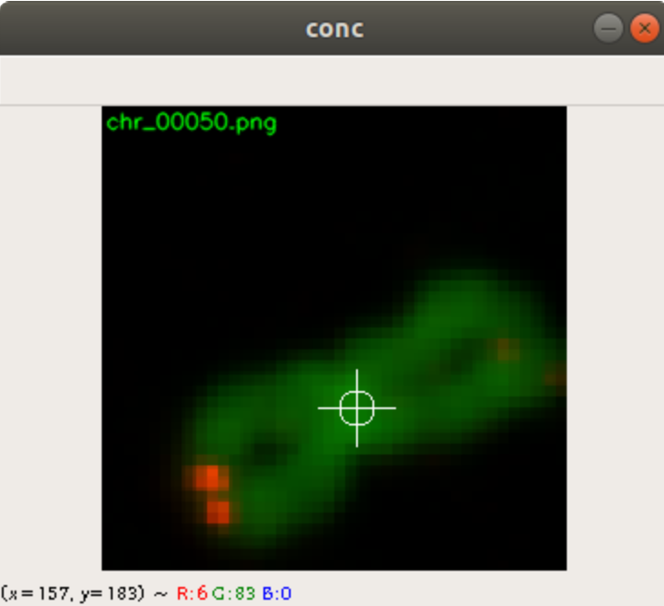
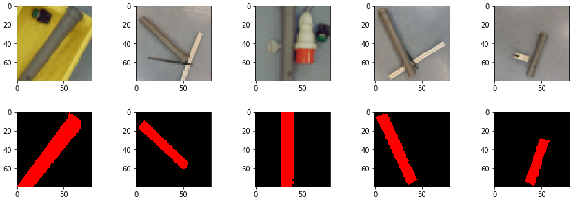
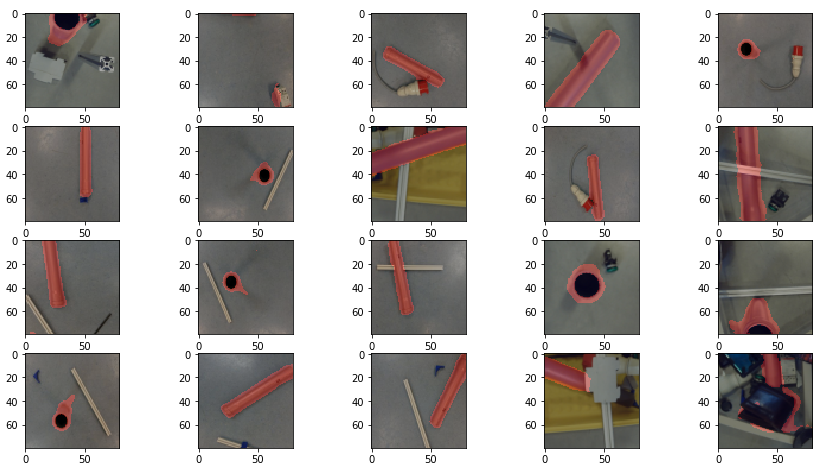
We tested the model with the code below. First, we loaded the image in the variable img with the opencv function imread read. Right after this, we have to take care of the image layers. The way opencv handles the image layers is different from the way Keras with its predict method does. They have the Red and the Blue layers switched. For this reason, we have to apply the cvtColor method, which switches the Red and Blue layers. The image is then normalized by dividing its pixels values with 255. Finally the prediction method is used to predict the image. Figure 4 shows an example of an image for input, which is printed out by the matplotlib function imshow. The method predict returns a probability vector predictions. The index with the highest value of the vector corresponds to the category. The category can be retrieved from the class_indices list.

img = cv2.imread(os.path.join(valid_path,"Apfel/cropped_img_592.jpg"),1)
img = cv2.cvtColor(img, cv2.COLOR_BGR2RGB)
imshow(img)   
img = np.array(img, dtype=np.float32)
img *= 1.0/255.0
predictions = model.predict([[img]])
print(predictions)
result = np.where(predictions[0] == np.amax(predictions[0]))
assert len(result)==1
print(list(valid_it.class_indices)[result[0][0]])

We tested a few times with different image and saw that the prediction delivered pretty good results.

Figure 4: Prediction Image

The Raspberry Pi application

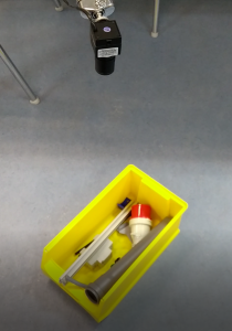
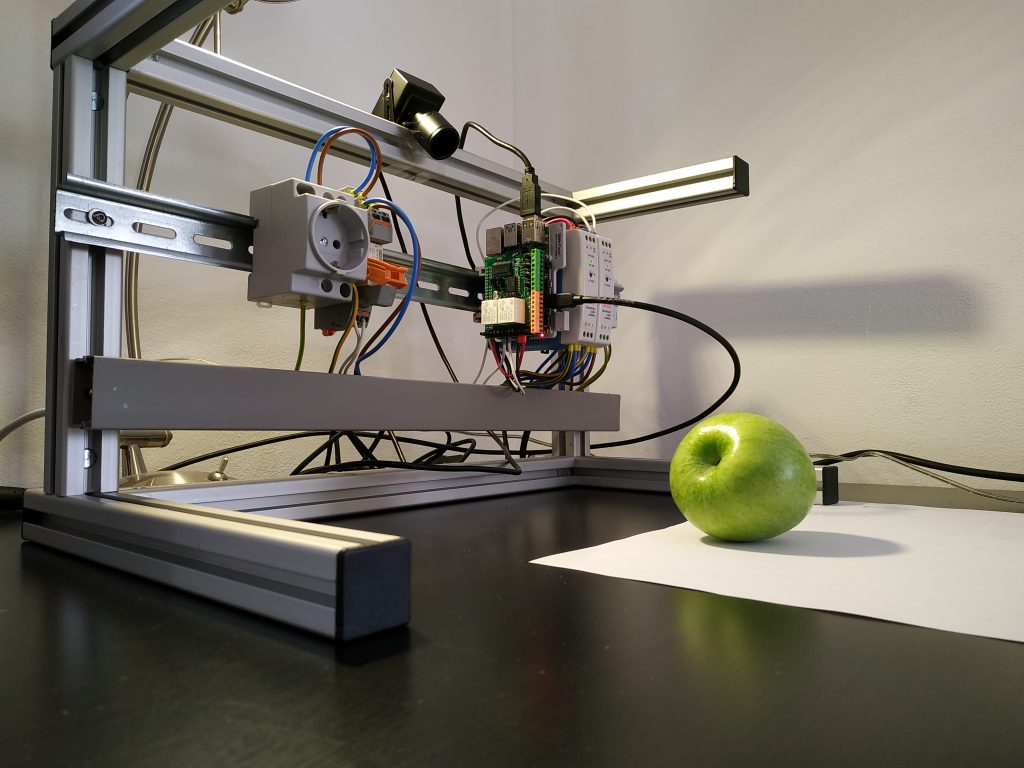
The setup of the experiment is shown in Figure 5. The raspberry pi 4, power supply and a socket are mounted on a top-hat rail. On the raspberry pi you see a piface shield attached. The shield had to be mechanically prepared to fit on a raspberry pi 4. The shield provides buttons in case it is needed. Additionally we have a relay and a power socket. The relay can be triggered by the piface, so the relay applies 230V to the socket. On top of the construction you find an usb camera.

Figure 5: Experiment Setup

We defined a function getCrop, see code below, which crops the image to the size of the portion of the fruit. This procedure was already explained above. Here we introduced the variable threshset, where the user can modify the threshold value of the opencv threshold method using keys. This is explained later.

threshset = 100

def getCrop(im):
    global threshset
    imgray = cv2.cvtColor(im, cv2.COLOR_BGR2GRAY)
    ret, thresh = cv2.threshold(imgray, threshset, 255, 0)
    contours, hierarchy = cv2.findContours(thresh, cv2.RETR_TREE, cv2.CHAIN_APPROX_SIMPLE)
    if len(contours) >= 1:
        cnts = sorted(contours, key=cv2.contourArea, reverse=True)    
        for cnt in cnts:
            x, y, w, h = cv2.boundingRect(cnt)
            if w > im.shape[0]*20//100 and w < im.shape[0]*95//100:
                if h > im.shape[1]*20//100 and h < im.shape[1]*95//100:
                    w = max((h, w))
                    h = w
                    return x,y,w
    return 0,0,0

In the beginning we faced the problem that the neural network did not predict very well due to too few training images. Therefore we introduced a function to save easily badly predicted images. The name of the function is saveimg. It simply saves an image img to a directory with a name containing the parameters dircat and fruit. The image name also contains the date and the time.

def saveimg(img, dircat, fruit):
    global croppedfolder
    now = datetime.now()
    dt_string = now.strftime("%d_%m_%Y_%H_%M_%S")
    resized =  np.zeros((image_size[0], image_size[1],3), np.uint8)
    resized = cv2.resize(img, image_size, interpolation = cv2.INTER_AREA)
    cv2.imwrite(os.path.join(croppedfolder, dircat, fruit, str("img_"+dt_string+".jpg")), resized)

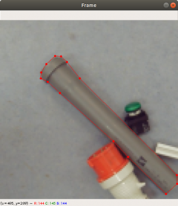
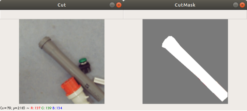
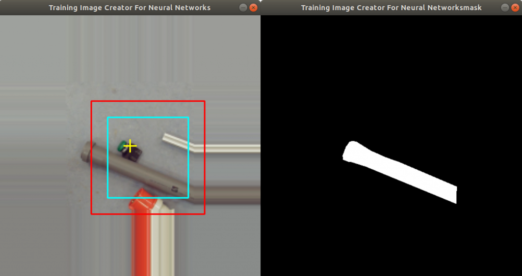
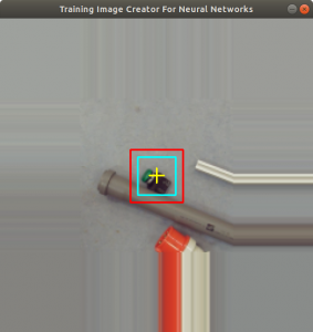
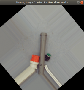
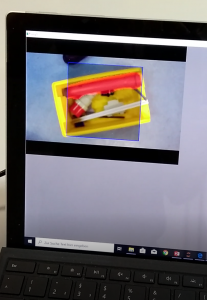
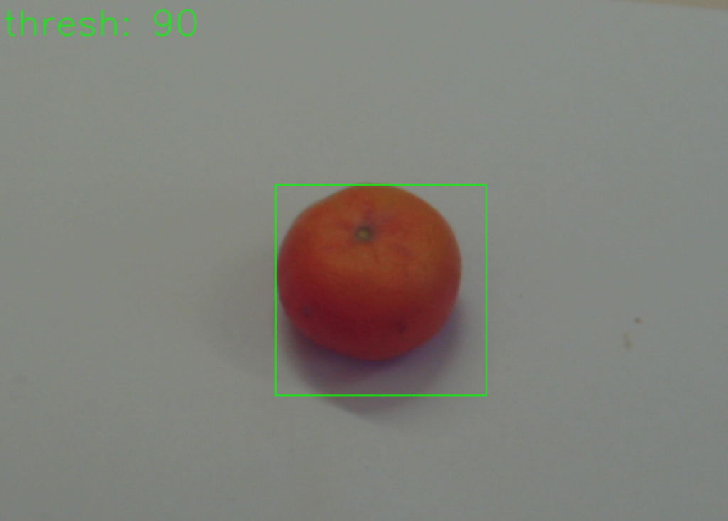
Below you find the raspberry pi application code. In the beginning it sets up the opencv video feature. Inside the while loop, an image frame from the usb camera is taken, which is then copied into the image objectfr. The function getCrop is used to get the fruit portion of the image and a rectangle is drawn around the fruit portion. The function putText writes the current value of threshset into the image objectfr as well. The application then shows the modified image on a display, see Figure 6. The opencv method waitkey checks for a pressed key. In case a key was pressed, code depending on the key will be executed.

cam = cv2.VideoCapture(0)
cv2.namedWindow("object")

while True:
    ret, frame = cam.read()
    if not ret:
        print("cam.read something wrong")
        break
    objectfr = frame.copy()
    x,y,w = getCrop(objectfr)
    cv2.rectangle(objectfr, (x,y), (x+w,y+w), (0,255,0), 1)
    cv2.putText(objectfr, "thresh: {}".format(threshset), (10,30),  cv2.FONT_HERSHEY_SIMPLEX, 1, (0, 255, 0), 1, cv2.LINE_AA)
    cv2.imshow("object", objectfr)
    if not ret:
        break
    k = cv2.waitKey(1)
    if k & 0xFF == ord('q') :
        break
    elif k & 0xFF == ord('n') :
        resized =  np.zeros((image_size[0], image_size[1],3), np.uint8)
        resized = cv2.resize(frame[y:y+w,x:x+w,:], image_size, interpolation = cv2.INTER_AREA) 
        cv2.imwrite("checkpic.jpg",resized)
        resized = cv2.cvtColor(resized, cv2.COLOR_BGR2RGB)
        resized = np.array(resized, dtype=np.float32)
        resized *= 1.0/255.0
        predictions = model.predict([[resized]])
        print(predictions)
        result = np.where(predictions[0] == np.amax(predictions[0]))
        assert len(result)==1
        print(result[0][0])
        print(list(valid_it.class_indices)[result[0][0]])
        os.system("espeak -vde {}".format(list(valid_it.class_indices)[result[0][0]]))
    elif k & 0xFF == ord('a'):
        saveimg(frame[y:y+w,x:x+w,:], "Training", "Apfel")
        img_counter += 1
    elif k & 0xFF == ord('z'):
        saveimg(frame[y:y+w,x:x+w,:], "Training", "Zwiebel")
        img_counter += 1
    elif k & 0xFF == ord('o'):
        saveimg(frame[y:y+w,x:x+w,:], "Training", "Orange")
        img_counter += 1                
    elif k & 0xFF == ord('k'):
        saveimg(frame[y:y+w,x:x+w,:], "Training", "Kartoffel")
        img_counter += 1
    elif k & 0xFF == ord('+'):
        threshset += 5
        if threshset > 255:
            threshset = 255
    elif k & 0xFF == ord('-'):
        threshset -= 5
        if threshset < 0:
            threshset = 0
        
        
cam.release()
cv2.destroyAllWindows()

If the key ‘q’ is pressed, than the application stops. If the key ‘n’ is pressed, the image inside the rectangle is taken and the category is predicted with the Keras predict method. The string is handed over to the espeak application which speaks out the category on the speaker attached on the raspberry pi. The keys ‘a’, ‘z’, ‘o’, ‘k’ execute the saveimg function with different parameters. The purpose of these keys is, that the user can save an image, in case there is a bad prediction. Next time, the model is trained, the saved image will be included in the training data. At last we have the ‘+’ and ‘-‘ keys, which modify the threshset value. The effect will be, that the rectangle (Figure 6, green rectangle) is enlarged or downsized due to the shadow on the background.

Figure 6: Displayed Image

Conclusion

The application works amazingly well with few fruits to predict considering the relative low number of training data. In the beginning we had to retrain the model a couple of times with newly generated images using the application keys described above.

As soon as we take e.g. an apple with different colors, there is a high chance that the prediction fails. In such cases we have take more images and retrain again.

Acknowledgement

Thanks to Carmen Furch and Armin Weisser providing the data preparation code and the raspberry pi application.

Also special thanks to the University of Applied Science Albstadt-Sigmaringen offering a classroom and appliances to enable this research.

Centromere Position on a Chromosome Image using a Neural Network

Chromosomes have one short arm and one long arm. The centromere sits in between and links both arms together. Biologists find it convenient that an application can spot automatically the position of the centromere on a chromosome image. In general for image processing, it is useful for an application to know the centromere position to simplify the classification of the chromosome type.

With this project we want to show how an application can get the centromere positions by using a neuronal network. In order to train the neuronal network, we need sufficient training data. We show here, how we created the training data. A position in an image is a coordinate with two numbers. The application must therefore use an neuronal network with an regression layer as an output. In this post we show what kind of neuronal network we used for retrieving a position from an image.

Creating the Training Data

Previously we created with a tool around 3000 images from several complete chromosome images. We do not go much into detail about this tool. The tool works in a way that it loads in and shows a complete chromosome image with its 46 chromosomes and as an user we can select with the mouse a square on this image. The content of the square is then saved as a 128×128 chromosome image and as a 128×128 telomere image. Figure 1 shows an example of both images. We have created around 3000 chromosome and telomere images from different positions.

Figure 1: Chromosome Image and Telomere Image

Each time we save the chromosome and telomere images, the application updates a csv file with the name of the chromosome (chrname) and the name of the telomere (telname) using the write function of the code below. It uses the library pandas to concat rows to the end of a csv file with the name f_name.

def write(chrname, telname, x, y): 
  
    if isfile(f_name): 
  
        df = pd.read_csv(f_name, index_col = 0) 
        data = [{'chr': chrname, 'tel': telname, 'x': x, 'y':y}] 
        latest = pd.DataFrame(data) 
        df = pd.concat((df, latest), ignore_index = True, sort = False) 
    else: 
        data = [{'chr': chrname, 'tel': telname, 'x': x, 'y':y}] 
        df = pd.DataFrame(data) 

    df.to_csv(f_name) 

In the code above, you can see that a x and a y value is stored into the csv file, as well. This is the position of the centromere of the chromosome on the chromosome image. At this point of time, the position is not known yet. We need a tool, where we can click on each image to mark the centromere position. The code of the tool is shown below. There are two parts. The first part is the callback function click. It is called as soon as the user of the application presses a mouse button or moves the mouse. If the left mouse button is pressed, then the actual mouse position on the conc window is moved to the variable refPt. The second part of the tool loads in the a chromosome image from a directory chrdestpath and a telomere image from a directory teldestpath into a window named conc. The function makecolor (this function is described below) adds both images together to one image. The user can select with the mouse the centromere position and a cross appears on the clicking position, Figure 2. The application stores the position refPt by pressing the key “s” into the pandas data frame df. After this, the application loads in the next chromosome image from the directory chrdestpath and the next telomere image from the directory teldestpath.

refPt = (0,0)
mouseevent = False
def click(event,x,y,flags,param):
    global refPt
    global mouseevent
    if event == cv2.EVENT_LBUTTONDOWN:
        refPt = (x,y)
        mouseevent = True

cv2.namedWindow('conc')
cv2.setMouseCallback("conc", click)

theEnd = False
theNext = False

img_i=0
imgstart = 0
assert imgstart < imgcount

df = pd.read_csv(f_name, index_col = 0) 

for index, row in df.iterrows():
 
    if img_i < imgstart:
        img_i = img_i + 1
        continue
        
    chrtest = cv2.imread("{}{}".format(chrdestpath,row["chr"]),1)
    teltest = cv2.imread("{}{}".format(teldestpath,row["tel"]),1)
    
    conc = makecolor(chrtest, teltest)
    concresized = np.zeros((conc.shape[0]*2, conc.shape[1]*2,3), np.uint8)
    concresized = cv2.resize(conc, (conc.shape[0]*2,conc.shape[1]*2), interpolation = cv2.INTER_AREA)
    
    refPt = (row["y"],row["x"])
    cv2.putText(concresized,row["chr"], (2,12), cv2.FONT_HERSHEY_SIMPLEX, 0.4, (0, 255, 0), 1, cv2.LINE_AA)

    while True:
        cv2.imshow('conc',concresized)
        key = cv2.waitKey(1)
        if mouseevent == True:
            print(refPt[0], refPt[1])
            concresized = cross(concresized, refPt[0], refPt[1], (255,255,255))
            mouseevent = False
        if key & 0xFF == ord("q") :
            theEnd = True
            break
        if key & 0xFF == ord("s") :
            df.loc[df["chr"] == row["chr"], "x"] = refPt[1]//2
            df.loc[df["chr"] == row["chr"], "y"] = refPt[0]//2
            theNext = True
            break
        if key & 0xFF == ord("n") :
            theNext = True
            break
    if theEnd == True:
        break
    if theNext == True:
        theNext = False
           
df.to_csv(f_name) 
cv2.destroyAllWindows()

Figure 2 shows the cross added to the centromere position selected by the user. This procedure was done around 3000 times on chromosome and telomere images, so the output was a csv file with 3000 chromosome image names, telomere image names, and centromere positions.

Figure 2: Centromere Postion on a Chromosome Image

Augmenting the Data

In general 3000 images are too few images to train a neuronal network, so we augmented the images to have more training data. This was done by mirrowing all chromosome images (and its centromere positions) on the horizontal axis and on the vertical axis. This increased the number of images to 12000. The code below shows the load_data function to load the training data or validation_data into arrays

def load_data(csvname, chrdatapathname, teldatapathname):
    X_train = []
    y_train = []
    
    assert isfile(csvname) == True
    df = pd.read_csv(csvname, index_col = 0) 
    for index, row in df.iterrows():
                          
        chrname = "{}{}".format(chrdatapathname,row["chr"])
        telname = "{}{}".format(teldatapathname,row["tel"])
    
        chrimg = cv2.imread(chrname,1)
        telimg = cv2.imread(telname,1)                  
                 
        X_train.append(makecolor(chrimg, telimg))
        y_train.append((row['x'],row['y']))
    return X_train, y_train

In the code above you find a makecolor function. makecolor copies the grayscale images of the chromosome into the green layer of a new color image and the telomere image into the red layer of the same color image, see code of the function makecolor below.

def makecolor(chromo, telo):

    chromogray = cv2.cvtColor(chromo, cv2.COLOR_BGR2GRAY)
    telogray = cv2.cvtColor(telo, cv2.COLOR_BGR2GRAY)
    
    imgret = np.zeros((imgsize, imgsize,3), np.uint8)
    
    imgret[0:imgsize, 0:imgsize,1] = chromogray
    imgret[0:imgsize, 0:imgsize,0] = telogray
    
    return imgret

Below the function code mirrowdata to flip the images horizontally or vertically. It uses the parameter flip to control the flipping of the image and its centromere position.

 def mirrowdata(data, target, flip=0): 
    xdata = []
    ytarget = []

    for picture in data:
        xdata.append(cv2.flip(picture, flip))
        
    for point in target:
        if flip == 0:
            ytarget.append((imgsize-point[0],point[1]))
        if flip == 1:
            ytarget.append((point[0],imgsize-point[1]))
        if flip == -1:
            ytarget.append((imgsize-point[0],imgsize-point[1]))
    
    return  xdata, ytarget

The following code loads in the training data into the array train_data and the array train_target. train_data contains color images of the chromosomes and telomeres and train_target contains the centromere positions. The mirrowdata function is applied twice on the data with different flip parameter settings. After this, the data is converted to numpy arrays. This needs to be done to be able to normalize the images with the mean function and the standard deviation function. This is done for 10000 images among the 12000 images for the training data. The same is done with the remaining 2000 images for the validation data.

train_data, train_target = load_data(csvtrainname, chrtrainpath, teltrainpath)
train_mirrow_data, train_mirrow_target = mirrowdata(train_data, train_target, 0)
train_data = train_data + train_mirrow_data
train_target = train_target + train_mirrow_target
train_mirrow_data, train_mirrow_target = mirrowdata(train_data, train_target, 1)
train_data = train_data + train_mirrow_data
train_target = train_target + train_mirrow_target

train_data = np.array(train_data, dtype=np.float32)
train_target = np.array(train_target, dtype=np.float32)

train_data -= train_data.mean()
train_data /= train_data.std()

Modeling and Training the Neuronal Network

Since we have images we want to feed into the neural network, we decided to use a neuronal network with convolution layers. We started with a Layer having 32 filters. As input for training data we need images with size imgsize, which is in our case 128. After each convolution layer we added the max pooling function with pool_size=(2,2) which reduces the size of the input data by half. The output is fed into the next layer. Altogether we have four convolution layers. The number of filters, we increase after each layer. After the fourth layer we flatten the network and feed this into the first dense layer. Then we feed the output into the second dense layer having only two neurons. The activation function is a linear function. This means, we will receive two float values, which is supposed to be the position of the centromere. As a loss function we decided to use the mean_absolute_percentage_error.

model = Sequential()
model.add(Conv2D(32, (3, 3), activation='relu', kernel_initializer='he_uniform', kernel_regularizer=l2(0.01), bias_regularizer=l2(0.01), padding='same', input_shape=(imgsize, imgsize, 3)))
model.add(MaxPooling2D((2, 2)))
model.add(Conv2D(32, (3, 3), activation='relu', kernel_initializer='he_uniform', kernel_regularizer=l2(0.01), bias_regularizer=l2(0.01), padding='same'))
model.add(MaxPooling2D((2, 2)))
model.add(Conv2D(64, (3, 3), activation='relu', kernel_initializer='he_uniform', kernel_regularizer=l2(0.01), bias_regularizer=l2(0.01), padding='same'))
model.add(MaxPooling2D((2, 2)))
model.add(Conv2D(128, (3, 3), activation='relu', kernel_initializer='he_uniform', kernel_regularizer=l2(0.01), bias_regularizer=l2(0.01), padding='same'))
model.add(MaxPooling2D((2, 2)))
model.add(Flatten())
model.add(Dense(128, activation='relu', kernel_initializer='he_uniform'))
model.add(Dropout(0.1))
model.add(Dense(2, activation='linear'))
opt = Adam(lr=1e-3, decay=1e-3 / 200)
model.compile(loss="mean_absolute_percentage_error", optimizer=opt, metrics=['accuracy'])

We start the training with the fit method. The input parameters are the list of colored and normalized chromosome images (train_data), the list of centromere positions (train_target), and the validation data (valid_data, valid_target). A callback function was defined to stop the training as soon as there is no progress seen. Also checkpoints are saved automatically, e.g. if there is progress during the training.

callbacks = [
    EarlyStopping(patience=10, verbose=1),
    ReduceLROnPlateau(factor=0.1, patience=3, min_lr=0.00001, verbose=1),
    ModelCheckpoint('modelregr.h5', verbose=1, save_best_only=True, save_weights_only=True)
]

model.fit(train_data, train_target, batch_size=20, nb_epoch=50, callbacks=callbacks, verbose=1, validation_data=(valid_data, valid_target) )

The training took around five minutes on a NVIDIA 2070 graphics card. The accuracy is 0.9462 and the validation accuracy is 0.9258. This shows a small overfitting. The loss function shows the same overfitting result.

Testing

We kept a few chromosome images and telomere images aside for testing and predicting. The images were stored in a test_data array and normalized before prediction. The prediction was done with the following code.

predictions_test = model.predict(test_data, batch_size=50, verbose=1)

prediction_test contains now all predicted centromere positions. Figure 3 shows the positions added to the chromosome images. We can see that the position of the cross is pretty close to the centromere. However there are deviations.

Figure 3: Predicted centromere positions

For displaying the chromosomes as shown as in Figure 3 we use the following showpics function. Note in case you want to use this code, you have to be aware that the input images may not be normalized, otherwise you see see a black image.

def showpics(data, target, firstpics=0, lastpics=8):
    chrtail=[]
    pnttail=[]
    columns = 4
    print(data[0].shape)
    for i in range(firstpics, lastpics):
        chrtail.append(data[i])
        pnttail.append(target[i])
    rows = (lastpics-firstpics)//columns
    fig=figure(figsize=(16, 4*rows))
    for i in range(columns*rows):
        point = pnttail[i]
        fig.add_subplot(rows, columns, i+1)
        pic = np.zeros((chrtail[i].shape[0], chrtail[i].shape[1],3), np.uint8)
        pic[0:pic.shape[0], 0:pic.shape[1], 0] = chrtail[i][0:pic.shape[0], 0:pic.shape[1], 0]
        pic[0:pic.shape[0], 0:pic.shape[1], 1] = chrtail[i][0:pic.shape[0], 0:pic.shape[1], 1]
        pic[0:pic.shape[0], 0:pic.shape[1], 2] = chrtail[i][0:pic.shape[0], 0:pic.shape[1], 2]
        imshow(cross(pic, int(point[1]), int(point[0]), (255,255,255)))    

Conclusion

The intention of this project was to show how to use linear regression as the last layer of the neuronal network. We wanted to get a position (coordinates) from an image.

Firstly we marked about 3000 centromere positions of chromosomes and telomere images with a tool we created. Then we augmented the data to increase the data to 12000 images. We augmented the data by horizontal and vertical flipping.

Secondly we trained a multilayer convolutional neural network with four convolutional layers and two dense layers. The last dense layer has two neurons. One for each coordinate.

The prediction result was fairly good, considering the little effort we used to optimize the model. On Figure 3 we still can see that the centromere position is not always hit on the right spot. We expect improvement after we will add more data and optimize the model.

Cheat Check for Take Home Exams with Deep Learning

Many schools have an honor code system, which prevents very often the cheating during exams and tests among students. Students simply do not show their exams and tests to other students who are trying to cheat. One reason why students do not let to cheat can be the consequences of violating the honor code, which can be very harsh and result often to the exclusion from the school. Another reason is definitively the mindset of many students about this topic. Their opinion about the purpose of exams and tests is just to proof the knowledge and to get recognition from the professor in form of a grade. In my experience both are the main reasons why take home exams (even closed book) can work very well in schools having the honor code system.

Other schools do not have such an honor code system. The consequences of cheating during tests and exams is much less drastic. Being caught while cheating will just lead to the exclusion from the exam, which can be repeated the next semester. In some cases it will just lead to downgrade the grade. The mindset of some (but not all) students is very different, as well. Cheating is widely considered as helping.

On the one side the none existence of the honor code system makes the use of take home exams very difficult. On the other side, take home exams do have advantages for both, the students and the professors. Students can proof their knowledge not only in 1.5 hours but can take their time for one day, or a week. So the quality of the turned in exams is in general much better. Still, there is no way to prevent, that students exchange information with each other. Which is actually not necessarily a bad thing, because in real life this is just the usual case. So what we do is to accept the exchange of information, but we do not accept the copying of sentences and text paragraphs or modifying them. However, if we have 60 exams with 20 pages each, there is almost no way to control copying. Unless we use electronic help.

The Idea: Using an overfitted neural network

In our classes, students need to turn in the take home exams not only in paper form, but also in electronic form, such as a PDF files. The application we wrote reads in the PDF files and stores its sentences in a list which represents the training data. The training data is then fed into a neural network for training. In general neural networks are used for prediction. A commonly used example are cinema reviews. The application feeds the trained neural network with a cinema reviews and the neural network categorizes them as a positive or as a negative review. This is a prediction use case. Overfitting during neural network training is here not the right thing to do. In our case, we do not want prediction. If we feed a sentence to the trained neural network, we want to know to which student the sentences belongs to. So what we need is a neural network, which learned the sentences and categorizes them to students to which they belong to. Learning of sentences can be done with overfitting.

Loading in the training data

Students have to turn in the exams as PDF files. PDF files in general do not have the right format to be processed by an application. Like so often in data science, we need to bring the files into a form which can be handled with a neural network. Unfortunately this can be a very tedious work. Fortunately there is a Linux program called pdftotext which converts PDF files into text. So first thing is to convert all turned in PDF files and the PDF file of the assignment itself into text files.

Here comes the problem, for which I do not have a good solution yet. Figure 1 shows a table of a PDF file. This is a table of a turned in take home exam.

Figure 1: Table from a take home exam

The program pdftotext converts very well PDF text passage into a text file, but the text of PDF tables is aligned in a way, which is difficult to parse, because we do not know to which column a sentence belongs to, see the Figure 2. You can see that here are three columns descriptions: “Nr.”, “Beschreibung der Tätigkeiten” and “Geschätztes Datum der Lieferung”. The column descriptions are just written into one line (see green line). The same is true for the following table rows (see turquoise lines), which are just written into one line, as well.

Figure 2: Converted table from PDF to text

Ideally the text files should list the sentences one after the other, separated by a carriage return. However pdftotext does not do this, especially with tables. Before writing an application to convert the pdftotext generated text file into the needed format, we decided to do this step manually. It is left for future to write such an application.

We tediously edited the pdftotext generated text files of each take home exam in a way, that all sentences are listed one after the other, see Figure 3. Actually, this doing this work has the advantage, that we get an impression about the turned in take home exams before actually correcting and grading them. So editing and correcting can be done in parallel.

Figure 3: Text file with sentences in list

The following source code loads a text file and its sentences into the list onedoc, and then appends it to the list documents. So all sentences in the list documents can addressed with two indices representing the text file number and the sentence number. During this process each sentence is stripped off from special characters, non-ascii characters and digits. All character are converted to lower case.

def remove_non_ascii(text):
    return ''.join([i if ord(i) < 128 else ' ' for i in text])

def remove_digit(text):
    return ''.join([i if not i.isdigit() else ' ' for i in text])

pathname='/home/inf/Daten/CPCHECK/WS1920/train'
sentences = []
documents = []
categories = []
numbertodoc = {}

maxlength = 0
documentnumber=0
 
for f in os.listdir(pathname):
    if f.endswith('.txt'):
        name = os.path.join(pathname,f)
        onedoc = []
        with open(name) as fp:
            line = fp.readline()
            cnt = 1
            while line:
                line = line.strip()
                if len(line) != 0:
                    line = line.lower()
                    line = line.replace('\\', ' ').replace('/', ' ').replace('|', ' ').replace('_', ' ')
                    line = line.replace('ä', 'ae').replace('ü', 'ue').replace('ö', 'oe').replace('ß', 'ss')
                    line = line.replace('+', ' ').replace('-', ' ').replace('*', ' ').replace('#', ' ')
                    line = line.replace('\"', ' ').replace('§', ' ').replace('$', ' ').replace('%', ' ').replace('&', ' ')
                    line = line.replace('(', ' ').replace(')', ' ').replace('{', ' ').replace('}', ' ')
                    line = line.replace('[', ' ').replace(']', ' ').replace('=', ' ').replace('<', ' ').replace('>', ' ')
                    line = line.replace('i. h. v.', 'ihv').replace('u. u.', 'uu').replace('u.u.', 'uu')
                    line = line.replace('z. b.', 'zb').replace('z.b.', 'zb')
                    line = line.replace('d. h.', 'dh').replace('d.h.', 'dh').replace('d.h', 'dh')
                    line = line.replace('o.ae.', 'oae').replace('o. ae.', 'oae')
                    line = line.replace('u.a.', 'ua').replace('u. a.', 'ua')                 
                    line = line.replace('ggfs', 'ggf')
                    line = remove_non_ascii(line)
                    line = remove_digit(line) 

                    line = line.replace('.', ' ').replace(',', ' ').replace('!', ' ').replace('?', ' ').replace(':', ' ').replace(';', ' ')
                    sentences.append(line.split())
                    onedoc.append(line.split())
                    if len(sentences[-1]) > maxlength:
                        maxlength = len(sentences[-1])
                    cnt += 1
                line = fp.readline()
            documents.append(onedoc)
            numbertodoc[documentnumber] = os.path.basename(name)
            documentnumber += 1

for catnum in range(documentnumber):
    category = [0.0] * documentnumber
    category[catnum] = 1.0
    categories.append(category)
    

The list categories in the source code above consists of a list of vectors. The vector’s length is the number of take home exams. Each vector categorizes the owner of the take home exam with the position of the element having a 1.0. E.g. the first element of the vector is 1.0 and the remaining elements are 0.0, and the vector points to the first take home exam owner. These vectors are needed as input to the neural network to categorize each sentence of one take home exam.

A third list called sentences is needed later to create a vocabulary and to embed the words. All sentences of all take home exams are appended into this list.

Creating a vocabulary and embedding the words

Let us take a look at the sentence from above: ” Im Folgenden sind Tätigkeiten des Auftraggebers aufgeführt “. It is a German sentence which makes sense (the meaning is completely irrelevant). The words of the sentence make sense because the words can be seen in a context. There are existing libraries which can group words used in a context (or sentence) with vectors. So each word can be represented by a n-dimensional vector and all the vectors of one sentences can be grouped by pointing them into similar directions. Same is true for all sentences of each take home exam. Vectors can be appointed to each word. All words used in a similar context point into similar directions. This is also called word embedding. The code below generates the vocabulary and embeds all words inside the list sentences. Word2Vec from the gensim library assigns each word a 50-dimensional vector and returns an Word2Vec model:

EMBEDDED_DIM = 50
model = Word2Vec(sentences, min_count=1, size=EMBEDDED_DIM)

The code below shows how each word from the Word2Vec model vocabulary is assigned to two dictionaries. The method keys is returning the list of words of the created vocabulary. In tokendict each word from the model is assigned a value. Correspondingly, in worddict each value is assigned to a word from the model, so now we have a word-value and a value-word mapping. Conversions in both directions are needed because a neural network must be fed with numbers and not with words.

tokendict = {}
tokendict['noword']=0
worddict = {}
worddict[0]='noword'

i=1
for key in model.wv.vocab.keys():
    tokendict[key]=i
    worddict[i]=key
    i+=1

Creating the training data set

For training we need both the sentences of the take home exams and the categories as vectors. The category vectors assign an owner to each sentence. The sentences cannot be fed with words into the neuronal network, so we need to convert the words into numbers. The assignments of words to values have already been done above (tokendict and worddict). Sentences differ in lengths. But neural networks need fixed size data as input. We can assume that the maximum length of a sentence is less that 100 words. This can also be verified very easily during the data loading. So the words inside the documents array are assigned to values (using tokendict and worddict) and appended to a list x_train. x_train is set to a fixed size (in this case 100). All elements of x_train exceeding the size of the sentence are padded to 0 (which has the ‘noword’ assignment). The keras method pad_sequences is exactly doing this. Below the code creates training data.

x_train = []
y_train = []

for i in range(0, documentnumber):
    document = documents[i]
    for sent in document:
        tokensent = []
        for word in sent:
            tokensent.append(tokendict[word])
        x_train.append(tokensent)
        y_train.append(categories[i])    

print(len(y_train))
x_train = pad_sequences(x_train, padding='post', maxlen=100)

Each sentence needs to be categorized to one take home exam owner. For this we assign the category vectors to the y_train list.

Compiling and training the model

All word vectors from the Word2Vec model have to be moved into a data structure which we call embedded_matrix. embedded_matrix is a two dimensional array with the size of the number of vocabulary and the size of the dimension of the word vectors (which is 50). The copying code is shown below:

embedding_matrix = np.zeros((len(model.wv.vocab)+1, EMBEDDED_DIM))
for i in range(1,len(model.wv.vocab)+1):
    embedding_matrix[i]=model[worddict[i]]

We added a one to the size of the vocabulary (first line in code above), because we count additionally the word ‘noword’. The embedded_matrix can be represented as a layer of the neural network, with the element values of the word vectors as their weights. Keras provides a method Embedding to incorporate the embedding_matrix. See the next source code compiling the model:

modelnn = Sequential()
modelnn.add(layers.Embedding(len(model.wv.vocab)+1, EMBEDDED_DIM, weights=[embedding_matrix], input_length=100, trainable=True))
modelnn.add(layers.GlobalMaxPool1D())
modelnn.add(layers.Dense(100, activation='relu'))
modelnn.add(layers.Dense(documentnumber, activation='softmax'))
modelnn.compile(optimizer='adam',
              loss='categorical_crossentropy',
              metrics=['accuracy'])
modelnn.summary()

Note that the parameter trainable is set to True, because we want that the word vector elements can change during the training. We added two additional Layers with 100 neurons to the model. The last layer has exactly the number of take home exam participants (documentnumber). We chose softmax as an activation function. Therefor, if you count all output value of the last layer, it should result to one (which is not necessarily true for the sigmoid activation function). You can consider the output value as a probability that a sentence belongs to an owner. We chose the categorical cross entropy as a loss function, because we expect that one sentence can have several take home exam owners. This is exactly, what we want to figure out! The training is started with the following code:

y_train = np.array(y_train, dtype=np.float32)
modelnn.fit(x_train, y_train, epochs=40, batch_size=20)

The training takes about ten minutes on a NVIDIA 2070 graphics card. The accuracy is about 93%. We do not care about the validation_accuracy, because we do not bother about validating the model. We do want overfitting, because we are not predicting here anything. We simply want to know who are the owners of a input sentence.

Who copied from whom?

After training we can use the predict method of the neural network model with sentences from the documents list. These are same sentences we used for training. Actually we are not predicting anything here, even if we use the predict method. The purpose is to receive an output vector, having the size of number of participants, with probabilities in its elements. If the probabilities exceed a threshold, than there is a high chance, the sentences belongs to the owner identified by its index. Of course there can be several owners of one sentence. Below are some helper functions to print out the documents having similarities.

 def sentencesFromDocument(number):
    assert(number < documentnumber)
    sentences = []
    for sent in documents[number]:
        tokensent = []
        for word in sent:
            tokensent.append(tokendict[word])
        sentences.append(tokensent)
    return pad_sequences(sentences, padding='post', maxlen=100)

def probabilityVector(sentences):
    y_sent = [0]*documentnumber
    for sent in sentences:
        x_pred=[]
        x_pred.append(sent)
        x_pred = np.array(x_pred, dtype=np.int32)
        y_sent += modelnn.predict(x_pred)
    return y_sent

def similardocs(number, myRoundedList, thresh):
    cats = myRoundedList[0]
    str=""
    once = False
    for i in range(len(cats)):
        if cats[i] >= thresh:
            if i != number and once == False:
                once = True
            if i != number and once == True:
                str+="\n   {}: Doc: {} Sim: {}".format(i, numbertodoc[i], cats[i])
    return str

The function sentencesFromDocument is returning a list of sentences in form of vectors with key values from a specified (number) document. All vectors have the size 100. 100 is the maximum size of one sentence.

The function probabilityVector is returning a vector with elements representing the probability of owning a sentence. The sentence is the input parameter. The input parameter is the sentence to be fed into the predict method.

The function similardocs prints out all documents having high probabilities with same sentence. They need to exceed a threshold thresh which is delivered as a parameter.

Below the source code, which is calling the helper functions above with each document.

for i in range(documentnumber):
    mylist = probabilityVector(sentencesFromDocument(i))
    myRoundedList =  list(np.around(np.array(mylist),decimals=0))
    print("{}: {} ".format(i, numbertodoc[i])+similardocs(i, myRoundedList,9))

The output of the code can be seen it Figure 3. At row “9:” there seems to be a hit, meaning that file 20.txt and file 6.txt have similar sentences. At row “10:” it seems that the owner of file 40.txt, 47.txt and 5.txt worked very well together.

Figure 3: Extract from output

Conclusion

The program worked very well in finding similarities in sentences between the take home exam owners. However I do not really trust the output so I cross check the real exams. Figure 4 shows one exam having similar or identical sentences with a second exam from another participant. All sentences which are similar or identical are marked.

Figure 4: Marked sentences

Using the cheat check definitively gives a good pointer to exam owners who turned in similar sentences. So the assumption that the participants worked together is not far fetched.

One problem which still needs to be solved is the structure of text processed by the program pdftotext. Currently we need to put the text manually in order which is quite cumbersome. In future we need a tool which is doing this automatically.

PVC Pipe Recognition in Trash with Machine Learning

Introduction

The major work for recycling companies consist of sorting trash before processing it further. Usually recyclable trash is delivered in containers and employees in excavators sort out the parts such as electronics, metals, plastics etc. before moving them onto assembly lines. The assembly lines have additional sensors and machinery to sort the trash even further until it is finally shredded. The shredded trash is very often used as an energy source in the concrete industry.

Due to law regulations, there is a limit of chlorine substance inside burnable energy source. Since many plastics consist of polyvinyl chloride (PVC), which contains chlorine, the recycling company must take a lot of effort to sort out PVC from the trash in order to sell the shredded trash as an burnable energy source.

The idea of this project is to create an application, which takes life images from the content of a container and highlights the pieces of PVC trash on a monitor or on augmentation glasses worn by the employee. So the employee in the excavator gets help from the application, which is showing which pieces he has to sort out with his excavator, before moving the trash onto the assembly lines.

We introduce an application, which will use machine learning methods for highlighting the PVC trash pieces. Since objects from PVC can have many sizes and forms, we will limit our application in recognizing PVC pipes having gray color. Figure 1 is showing such a pipe. The application should highlight each pixel containing the PVC pipe with color, so it stands out of the picture.

Figure 1: PVC pipe

Segmenting PVC Pipe Regions using U-Net

Since the application is marking segments from the image, we are facing a segmentation problem. Segmentation problems are very often solved in machine learning with U-Nets. A description of U-Nets can be found here. Our description of the same U-Net, which is used in this work, can be found here.

So the application needs firstly to take real life images from a camera with scenes of trash, secondly to process the images with a trained U-Net model to receive the regions with PVC pipes and then thirdly to add the output image of the U-Net model with the original image. The output image is then displayed to the employee e.g. on a display. In Figure 2 you can see such a scene containing a PVC pipe.

Figure 2: Scene of trash

The items seen in Figure 2 will be used for training the U-Net model. So the next step is to generate many images of different configurations of item positions and light conditions for the model training.

There are two kind of images need to be fed into the U-Net model: the original image and the image containing a mask of the PVC pipe, indicating which pixel is a pipe, and which is not a pipe. We have therefore for each pixel two categories: pipe or not a pipe. So not only we need many original images but also we need many corresponding mask images. The mask images must be processed from the original images. In Figure 3 you can see what needs to be fed into the U-Net model for training, but the number of different kinds a images with different configurations needs to be in the thousands to get good results. The pixels of the mask image (right) in Figure 3 indicates if the pixel of the left image is a PVC pipe (white pixel) or not a PVC pipe (black pixel).

Figure 3: Original and mask image

Generating the training data set

I mentioned before that we need thousands of original and mask training images to get good results with training the model and with predicting the mask image from the trained model. In order to receive so many images, we need a strategy to create such a large number of images. Photographing thousands of scenes is possible, but very tedious. In order to receive the masks from the original image we need an ergonomic tool to create the masks in a very easy and fast way. Another strategy to improve the effort for gathering images is using an augmentation tool.

In this project, we programmed a tool, where the user can select the outline of the PVC pipe by clicking points on the original image. A polygon is create from the sequence of points, which is fed into the OpenCV function fillPoly to create the mask. Part of the source code is shown below:

pathnameimages = "/home/inf/Daten/Trash/images2/"
pathnamecuts = "/home/inf/Daten/Trash/train3/cuts/"
pathnamemasks = "/home/inf/Daten/Trash/train3/masks/"

def mouse_drawing(event, x, y, flags, params):
    global polygon
    global clicked
    if event == cv2.EVENT_LBUTTONDOWN:
        print("Left click:({},{})".format(x, y))
        polygon.append((x, y))
        clicked = True

dirlist = os.listdir(pathnameimages)

dirlist.sort()

fromto = (0,len(dirlist))

for i in range(fromto[0], fromto[1]):

    if stop == True:
        break
    print(dirlist[i])

    img = join(pathnameimages, dirlist[i])
    file = cv2.imread(img, 1)
    assert file.shape[0] == file.shape[1]
    img = np.zeros([file.shape[0]*2, file.shape[1]*2,3], dtype=np.uint8)       
    img = cv2.resize(file.copy(), (incshape[0], incshape[1]), interpolation = cv2.INTER_AREA) 
                    
    original = img.copy()

    polygon.clear()

    cv2.namedWindow("Frame")
    cv2.setMouseCallback("Frame", mouse_drawing)

    while True:
        
        cv2.imshow("Frame", img)
        key = cv2.waitKey(1)

        if key & 0xFF == ord("n"):
            break
                    
        if key & 0xFF == ord("q"):
            stop = True
            break                    
                    
        if key & 0xFF == ord("c") and len(polygon) > 0:
            cnt = np.array(polygon)
            mask = np.zeros(original.shape, dtype=np.uint8)
            cv2.fillPoly(mask, pts=[cnt], color=(255,255,255))

            masked_image = cv2.bitwise_and(original, mask)

            original = cv2.resize(original, (256, 256), interpolation=cv2.INTER_AREA)
            imgnorm = normalize(masked_image)
            imgnorm = cv2.resize(imgnorm, (256, 256), interpolation=cv2.INTER_AREA)

            cv2.namedWindow("Cut")
            cv2.imshow("Cut", original)
            cv2.namedWindow("CutMask")
            cv2.imshow("CutMask", imgnorm)

            cv2.waitKey(0)            

            imgnorm = imgnorm*255

            cv2.imwrite(pathnamecuts+str(i+IMG_NAME_START)+".png", original)
            cv2.imwrite(pathnamemasks+str(i+IMG_NAME_START)+".png", imgnorm)

            polygon.clear()

            cv2.destroyWindow("Cut")
            cv2.destroyWindow("CutMask")

        if clicked == True:
            cnt = np.array(polygon) 
            img = cv2.resize(file.copy(), (incshape[0], incshape[1]), interpolation = cv2.INTER_AREA) 

            if len(polygon) > 2:
                cv2.drawContours(img, [cnt], 0, (0, 0, 255), 1)

            for pnt in polygon:
                cv2.circle(img, pnt, 3, (0, 0, 255), -1)

            clicked = False
                    
cv2.destroyAllWindows()
stop = False

The code above reads in a list of images located in a directory (pathnameimages) and shows them in a window one by one. The user clicks with the mouse on the outline of the PVC pipe of the original image and each click shows a red dot on the display. If the user precedes until a polygon outlining the pipe is created. Figure 4 shows the completed outline of the pipe on the original image.

Figure 4: Selection of the PVC pipes outline

After the user completes marking the outline of the PVC pipe, he can press the key “c” and the tool generates two new images: the original image with the size needed by the U-Net model and the mask image, see Figure 5. Both images are saved to the training directories (here pathnamecuts and pathnamemasks). We have done this for around 500 images from different scenes. We took care that in some cases the PVC pipe is not shown in a scene, so there will be an empty mask.

Figure 5: Original image and mask image

Augmenting the training data

The effort to create 500 images from different scenes is pretty tedious and the number for training a U-Net is currently too low for good training and prediction results. So we decided to use a tool to create even more images by data augmentation. The user configures the tool by pointing the pathnames to the training and mask images directories. The tool then loads in the training and mask images one by one. Figure 6 shows the windows of the tool.

Figure 6: Augmentation tool

On the left side of Figure 6 you can see two squares added into the image: a red square (outer square) and a turquoise square (inner square). The region inside the turquoise square is cut out of the image and stored as an additional training image. The same is done with the mask image on the right side of Figure 6 (the squares are not shown here). The red square represents a boundary to indicate to the user that the turquoise square is not exceeding the boundary during rotation. In Figure 6 you can see, that the size of the image is actually enlarged. This is done by extending the first row, first column, last row and last column with the same pixel values. This is a simple data augmentation trick to prevent empty image regions, while the image is rotated. The user can adjust both square sizes by clicking the left and right mouse button. Figure 7 shows how the user has selected a smaller region.

Figure 7: Selection of a small region of interest

The user can start the data augmentation by pressing a key. The tool starts to rotate the turquoise square by ten degrees. Each time the turquoise square is rotated two new pictures are generated, one training image and one mask image, which are stored into the training data set. Figure 8 shows how the tool rotates the image. Additionally the image is flipped. Since we rotate the image by ten degrees and flip it each time, we produce 72 more images from the original training image. Since we have 500 images from different scenes, we produced now 36000 training and mask images. About 20% are moved to the validation data set and 5% to the test data set.

Figure 8: Image rotation

Training the U-Net model

First we need to load in the training and mask data, then we need to normalize the data. For data loading we provide the following two functions:

def load_cuts(pathname):
    X_train = []
    
    for f in os.listdir(pathname):
        if f.endswith('.png'):
            img = np.zeros([imgsize,imgsize,3],dtype=np.uint8)
            img = cv2.imread(os.path.join(pathname, f),1)
            assert img.shape == (imgsize, imgsize, 3)
            X_train.append(img)
        
    return X_train

def load_masks(pathname):
    y_train = []
    img_red = [[[0 for x in range(imgsize)] for y in range(imgsize)]  for z in range(3)]
  
    for f in os.listdir(pathname):
        if f.endswith('.png'):

            img_red = np.zeros([imgsize,imgsize,3],dtype=np.uint8)    
            img = cv2.imread(os.path.join(pathname, f),1)
            img_gray = cv2.cvtColor(img, cv2.COLOR_BGR2GRAY)
            assert img_gray.shape == (imgsize, imgsize)
            ret, img_red[:,:,2] = cv2.threshold(img_gray,200,255,cv2.THRESH_BINARY)
            y_train.append(img_red)
     
    return y_train

Both functions iterate through directories given by the pathname and append the images into lists. Mask images are gray scale images with three layers (BGR). The function load_masks is converting the gray scale image into an one layer gray scale image (OpenCV cvtColor function). The one layer gray scale image is the moved into the red layer of a new image (img_red). The other layers of img_red were set previously set to 0. Then the image is appended to the mask list. In Figure 9 you can see the training and the mask images.

Figure 9: Loaded training and mask images

The loaded training and masks images are then normalized by the following function calls:

X_train = np.array(X_train, dtype=np.float32)
y_train= np.array(y_train, dtype=np.float32)
cuts_valid = np.array(cuts_valid, dtype=np.float32)
masks_valid = np.array(masks_valid, dtype=np.float32)

X_train -= X_train.mean()
X_train /= X_train.std()
cuts_valid -= cuts_valid.mean()
cuts_valid /= cuts_valid.std()

y_train //= 255
masks_valid //= 255

X_train is the list of scene images. y_train is the list of masks. We moved about 20% of the scene images into the list cuts_valid which is used for validation. The corresponding 20% mask images are moved into masks_valid. X_train and cuts_valid are normalized by the mean function and standard deviation function. The mask lists (y_train and masks_valid) are normalized by division with 255.

The model is compiled with the binary cross entropy loss function. We chose for this function because there are only two categories a pixel can belong to. It is a pixel representing a PVC pipe and a pixel which is not a PVC pipe. Below the functions calls for compiling the U-Net model.

input_img = Input((im_height, im_width, 3), name='img')
model = get_unet(input_img, n_filters=16, dropout=0.05, batchnorm=True)
model.compile(optimizer=Adam(), loss="binary_crossentropy", metrics=["accuracy"])

Note that we use in the U-Net model a softmax activation function, because we have only two categories for each pixel: PVC pipe pixel and no PVC pipe pixel. The training is started with the fit function, see below. We use a callback function to store the model, if there is an improvement concerning loss.

callbacks = [
    EarlyStopping(patience=10, verbose=1),
    ReduceLROnPlateau(factor=0.1, patience=3, min_lr=0.00001, verbose=1),
    ModelCheckpoint('model-ct-1.h5', verbose=1, save_best_only=True, save_weights_only=True)
]

results = model.fit(X_train, y_train, batch_size=32, epochs=20, callbacks=callbacks, validation_data=(cuts_valid, masks_valid))

The training was continued until the accuracy had the value 0.9909 and the validation accuracy the value 0.9902. The loss function had the value 0.3636 and the validation loss function had the value 0.3658. These values show a small overfitting. The training was done on a NVIDIA 2070 graphics card. It took roughly ten minutes training time.

About 5% of the training images (mask images are not needed here) were put aside for test purpose. The code to predict mask images from training images can be seen below. The training images were appended into the X_test list and normalized. The method predict returns a list with predicted masks (predictions_test).

predictions_test = model.predict(X_test, batch_size=32, verbose=1)

Figure 10 shows a set of test images and below the test images the corresponding set of predicted mask images, returned by the predict method. Note that Figure 10 shows denormalized images, because predict returns normalized mask images.

Figure 10: Test images and predicted mask images

Test images and predicted mask images can be added together. The result will be an image which highlights the PVC pipe on the scene. See Figure 11.

Figure 11: Highlighted PVC pipes

The PVC pipe highlighter application

The application we wrote basically takes life images from a video of the scene with items. The images are fed into the predict method to generate a mask and finally adds the predicated image into the video stream. Figure 12 shows a setup with camera on the top and items on the bottom. Inside a box you find the PVC pipe. The application creates a video of the scene and each image of the video is fed into the predict method.

Figure 12: Camera taking life pictures

Figure 13 shows a snapshot of the video from the scene (Figure 12) with the predicted mask added. The pixels of the PVC pipe are highlighted with red color.

Figure 13: Life video of scene with items

Conclusion

In this project we created an application to highlight PVC pipes on images from a video. Each image is going through a prediction to create a prediction mask. Each pixel of the mask has two categories: a pixel can be a PVC pipe and a pixel can be no PVC pipe.

To produce masks we trained a U-Net model with training images from the scene. However mask images are needed as well, so they need to be created with a tool. We programmed an ergonomic tool where the user can click on the outline on the PVC pipe of the training image and a polygon is created. An OpenCV function returns the mask image from the polygon. Due to the tediousness of photographing so many training images we augment the images by rotation and flipping. So the number of original training images can multiplied by 72.

The application shows impressively how the PVC pipe is highlighted while the scene has defined items. Note we have perfect light conditions. As soon as new objects are put into the scene, they might be highlighted as well due to insufficient training and wrong prediction. Hence more real training data will be needed, and less training data generated from augmentation. Same is true with the light conditions. So more data is need from different light sources. A very easy thing to do is to augment the data with different contrast and brightness levels.

Ackowledgement

Special thanks to Jan Dieterich who provided the tool to augment the image data. Also special thanks to the University of Applied Science Albstadt-Sigmaringen offering a classroom and appliances to enable this research.