Introduction
The major work for recycling companies consist of sorting trash before processing it further. Usually recyclable trash is delivered in containers and employees in excavators sort out the parts such as electronics, metals, plastics etc. before moving them onto assembly lines. The assembly lines have additional sensors and machinery to sort the trash even further until it is finally shredded. The shredded trash is very often used as an energy source in the concrete industry.
Due to law regulations, there is a limit of chlorine substance inside burnable energy source. Since many plastics consist of polyvinyl chloride (PVC), which contains chlorine, the recycling company must take a lot of effort to sort out PVC from the trash in order to sell the shredded trash as an burnable energy source.
The idea of this project is to create an application, which takes life images from the content of a container and highlights the pieces of PVC trash on a monitor or on augmentation glasses worn by the employee. So the employee in the excavator gets help from the application, which is showing which pieces he has to sort out with his excavator, before moving the trash onto the assembly lines.
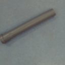
We introduce an application, which will use machine learning methods for highlighting the PVC trash pieces. Since objects from PVC can have many sizes and forms, we will limit our application in recognizing PVC pipes having gray color. Figure 1 is showing such a pipe. The application should highlight each pixel containing the PVC pipe with color, so it stands out of the picture.
Segmenting PVC Pipe Regions using U-Net
Since the application is marking segments from the image, we are facing a segmentation problem. Segmentation problems are very often solved in machine learning with U-Nets. A description of U-Nets can be found here. Our description of the same U-Net, which is used in this work, can be found here.
So the application needs firstly to take real life images from a camera with scenes of trash, secondly to process the images with a trained U-Net model to receive the regions with PVC pipes and then thirdly to add the output image of the U-Net model with the original image. The output image is then displayed to the employee e.g. on a display. In Figure 2 you can see such a scene containing a PVC pipe.
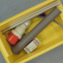
The items seen in Figure 2 will be used for training the U-Net model. So the next step is to generate many images of different configurations of item positions and light conditions for the model training.
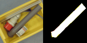
There are two kind of images need to be fed into the U-Net model: the original image and the image containing a mask of the PVC pipe, indicating which pixel is a pipe, and which is not a pipe. We have therefore for each pixel two categories: pipe or not a pipe. So not only we need many original images but also we need many corresponding mask images. The mask images must be processed from the original images. In Figure 3 you can see what needs to be fed into the U-Net model for training, but the number of different kinds a images with different configurations needs to be in the thousands to get good results. The pixels of the mask image (right) in Figure 3 indicates if the pixel of the left image is a PVC pipe (white pixel) or not a PVC pipe (black pixel).
Generating the training data set
I mentioned before that we need thousands of original and mask training images to get good results with training the model and with predicting the mask image from the trained model. In order to receive so many images, we need a strategy to create such a large number of images. Photographing thousands of scenes is possible, but very tedious. In order to receive the masks from the original image we need an ergonomic tool to create the masks in a very easy and fast way. Another strategy to improve the effort for gathering images is using an augmentation tool.
In this project, we programmed a tool, where the user can select the outline of the PVC pipe by clicking points on the original image. A polygon is create from the sequence of points, which is fed into the OpenCV function fillPoly to create the mask. Part of the source code is shown below:
pathnameimages = "/home/inf/Daten/Trash/images2/"
pathnamecuts = "/home/inf/Daten/Trash/train3/cuts/"
pathnamemasks = "/home/inf/Daten/Trash/train3/masks/"

def mouse_drawing(event, x, y, flags, params):
    global polygon
    global clicked
    if event == cv2.EVENT_LBUTTONDOWN:
        print("Left click:({},{})".format(x, y))
        polygon.append((x, y))
        clicked = True

dirlist = os.listdir(pathnameimages)

dirlist.sort()

fromto = (0,len(dirlist))

for i in range(fromto[0], fromto[1]):

    if stop == True:
        break
    print(dirlist[i])

    img = join(pathnameimages, dirlist[i])
    file = cv2.imread(img, 1)
    assert file.shape[0] == file.shape[1]
    img = np.zeros([file.shape[0]*2, file.shape[1]*2,3], dtype=np.uint8)
    img = cv2.resize(file.copy(), (incshape[0], incshape[1]), interpolation = cv2.INTER_AREA)

    original = img.copy()

    polygon.clear()

    cv2.namedWindow("Frame")
    cv2.setMouseCallback("Frame", mouse_drawing)

    while True:

        cv2.imshow("Frame", img)
        key = cv2.waitKey(1)

        if key & 0xFF == ord("n"):
            break

        if key & 0xFF == ord("q"):
            stop = True
            break

        if key & 0xFF == ord("c") and len(polygon) > 0:
            cnt = np.array(polygon)
            mask = np.zeros(original.shape, dtype=np.uint8)
            cv2.fillPoly(mask, pts=[cnt], color=(255,255,255))

            masked_image = cv2.bitwise_and(original, mask)

            original = cv2.resize(original, (256, 256), interpolation=cv2.INTER_AREA)
            imgnorm = normalize(masked_image)
            imgnorm = cv2.resize(imgnorm, (256, 256), interpolation=cv2.INTER_AREA)

            cv2.namedWindow("Cut")
            cv2.imshow("Cut", original)
            cv2.namedWindow("CutMask")
            cv2.imshow("CutMask", imgnorm)

            cv2.waitKey(0)

            imgnorm = imgnorm*255

            cv2.imwrite(pathnamecuts+str(i+IMG_NAME_START)+".png", original)
            cv2.imwrite(pathnamemasks+str(i+IMG_NAME_START)+".png", imgnorm)

            polygon.clear()

            cv2.destroyWindow("Cut")
            cv2.destroyWindow("CutMask")

        if clicked == True:
            cnt = np.array(polygon)
            img = cv2.resize(file.copy(), (incshape[0], incshape[1]), interpolation = cv2.INTER_AREA)

            if len(polygon) > 2:
                cv2.drawContours(img, [cnt], 0, (0, 0, 255), 1)

            for pnt in polygon:
                cv2.circle(img, pnt, 3, (0, 0, 255), -1)

            clicked = False

cv2.destroyAllWindows()
stop = False
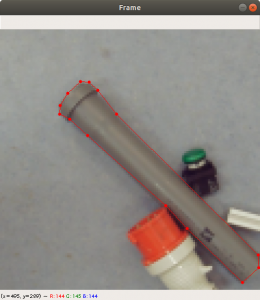
The code above reads in a list of images located in a directory (pathnameimages) and shows them in a window one by one. The user clicks with the mouse on the outline of the PVC pipe of the original image and each click shows a red dot on the display. If the user precedes until a polygon outlining the pipe is created. Figure 4 shows the completed outline of the pipe on the original image.
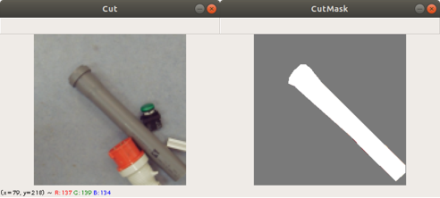
After the user completes marking the outline of the PVC pipe, he can press the key “c” and the tool generates two new images: the original image with the size needed by the U-Net model and the mask image, see Figure 5. Both images are saved to the training directories (here pathnamecuts and pathnamemasks). We have done this for around 500 images from different scenes. We took care that in some cases the PVC pipe is not shown in a scene, so there will be an empty mask.
Augmenting the training data
The effort to create 500 images from different scenes is pretty tedious and the number for training a U-Net is currently too low for good training and prediction results. So we decided to use a tool to create even more images by data augmentation. The user configures the tool by pointing the pathnames to the training and mask images directories. The tool then loads in the training and mask images one by one. Figure 6 shows the windows of the tool.
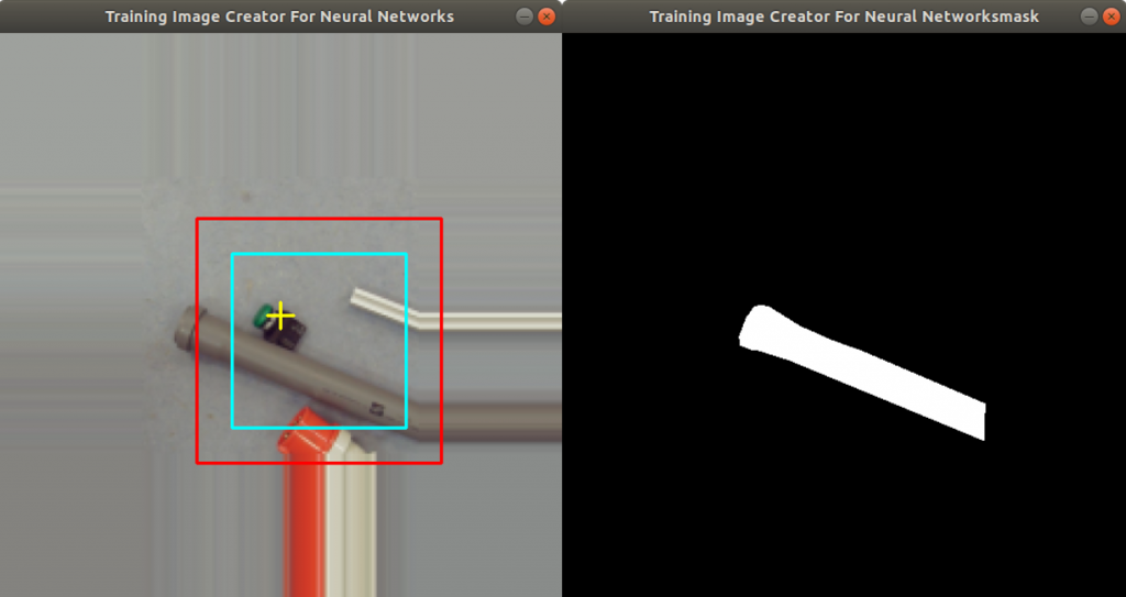
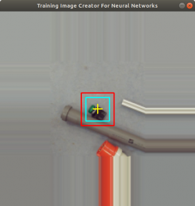
On the left side of Figure 6 you can see two squares added into the image: a red square (outer square) and a turquoise square (inner square). The region inside the turquoise square is cut out of the image and stored as an additional training image. The same is done with the mask image on the right side of Figure 6 (the squares are not shown here). The red square represents a boundary to indicate to the user that the turquoise square is not exceeding the boundary during rotation. In Figure 6 you can see, that the size of the image is actually enlarged. This is done by extending the first row, first column, last row and last column with the same pixel values. This is a simple data augmentation trick to prevent empty image regions, while the image is rotated. The user can adjust both square sizes by clicking the left and right mouse button. Figure 7 shows how the user has selected a smaller region.
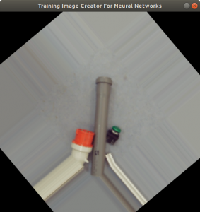
The user can start the data augmentation by pressing a key. The tool starts to rotate the turquoise square by ten degrees. Each time the turquoise square is rotated two new pictures are generated, one training image and one mask image, which are stored into the training data set. Figure 8 shows how the tool rotates the image. Additionally the image is flipped. Since we rotate the image by ten degrees and flip it each time, we produce 72 more images from the original training image. Since we have 500 images from different scenes, we produced now 36000 training and mask images. About 20% are moved to the validation data set and 5% to the test data set.
Training the U-Net model
First we need to load in the training and mask data, then we need to normalize the data. For data loading we provide the following two functions:
def load_cuts(pathname):
    X_train = []

    for f in os.listdir(pathname):
        if f.endswith('.png'):
            img = np.zeros([imgsize,imgsize,3],dtype=np.uint8)
            img = cv2.imread(os.path.join(pathname, f),1)
            assert img.shape == (imgsize, imgsize, 3)
            X_train.append(img)

    return X_train

def load_masks(pathname):
    y_train = []
    img_red = [[[0 for x in range(imgsize)] for y in range(imgsize)]  for z in range(3)]

    for f in os.listdir(pathname):
        if f.endswith('.png'):

            img_red = np.zeros([imgsize,imgsize,3],dtype=np.uint8)
            img = cv2.imread(os.path.join(pathname, f),1)
            img_gray = cv2.cvtColor(img, cv2.COLOR_BGR2GRAY)
            assert img_gray.shape == (imgsize, imgsize)
            ret, img_red[:,:,2] = cv2.threshold(img_gray,200,255,cv2.THRESH_BINARY)
            y_train.append(img_red)

    return y_train
Both functions iterate through directories given by the pathname and append the images into lists. Mask images are gray scale images with three layers (BGR). The function load_masks is converting the gray scale image into an one layer gray scale image (OpenCV cvtColor function). The one layer gray scale image is the moved into the red layer of a new image (img_red). The other layers of img_red were set previously set to 0. Then the image is appended to the mask list. In Figure 9 you can see the training and the mask images.
The loaded training and masks images are then normalized by the following function calls:
X_train = np.array(X_train, dtype=np.float32)
y_train= np.array(y_train, dtype=np.float32)
cuts_valid = np.array(cuts_valid, dtype=np.float32)
masks_valid = np.array(masks_valid, dtype=np.float32)

X_train -= X_train.mean()
X_train /= X_train.std()
cuts_valid -= cuts_valid.mean()
cuts_valid /= cuts_valid.std()

y_train //= 255
masks_valid //= 255
X_train is the list of scene images. y_train is the list of masks. We moved about 20% of the scene images into the list cuts_valid which is used for validation. The corresponding 20% mask images are moved into masks_valid. X_train and cuts_valid are normalized by the mean function and standard deviation function. The mask lists (y_train and masks_valid) are normalized by division with 255.
The model is compiled with the binary cross entropy loss function. We chose for this function because there are only two categories a pixel can belong to. It is a pixel representing a PVC pipe and a pixel which is not a PVC pipe. Below the functions calls for compiling the U-Net model.
input_img = Input((im_height, im_width, 3), name='img')
model = get_unet(input_img, n_filters=16, dropout=0.05, batchnorm=True)
model.compile(optimizer=Adam(), loss="binary_crossentropy", metrics=["accuracy"])
Note that we use in the U-Net model a softmax activation function, because we have only two categories for each pixel: PVC pipe pixel and no PVC pipe pixel. The training is started with the fit function, see below. We use a callback function to store the model, if there is an improvement concerning loss.
callbacks = [
    EarlyStopping(patience=10, verbose=1),
    ReduceLROnPlateau(factor=0.1, patience=3, min_lr=0.00001, verbose=1),
    ModelCheckpoint('model-ct-1.h5', verbose=1, save_best_only=True, save_weights_only=True)
]

results = model.fit(X_train, y_train, batch_size=32, epochs=20, callbacks=callbacks, validation_data=(cuts_valid, masks_valid))
The training was continued until the accuracy had the value 0.9909 and the validation accuracy the value 0.9902. The loss function had the value 0.3636 and the validation loss function had the value 0.3658. These values show a small overfitting. The training was done on a NVIDIA 2070 graphics card. It took roughly ten minutes training time.
About 5% of the training images (mask images are not needed here) were put aside for test purpose. The code to predict mask images from training images can be seen below. The training images were appended into the X_test list and normalized. The method predict returns a list with predicted masks (predictions_test).
predictions_test = model.predict(X_test, batch_size=32, verbose=1)
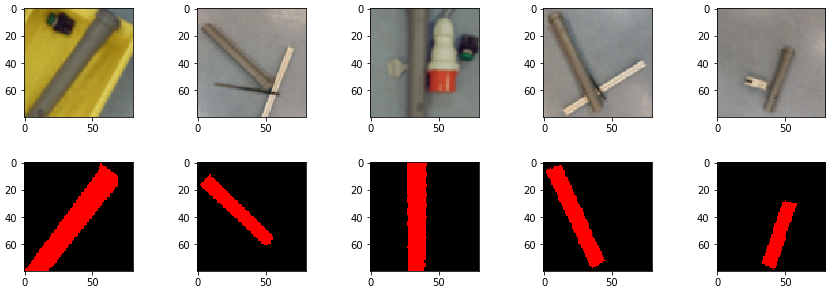
Figure 10 shows a set of test images and below the test images the corresponding set of predicted mask images, returned by the predict method. Note that Figure 10 shows denormalized images, because predict returns normalized mask images.

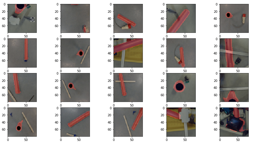
Test images and predicted mask images can be added together. The result will be an image which highlights the PVC pipe on the scene. See Figure 11.
The PVC pipe highlighter application
The application we wrote basically takes life images from a video of the scene with items. The images are fed into the predict method to generate a mask and finally adds the predicated image into the video stream. Figure 12 shows a setup with camera on the top and items on the bottom. Inside a box you find the PVC pipe. The application creates a video of the scene and each image of the video is fed into the predict method.
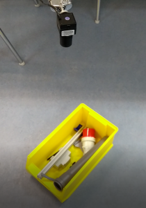
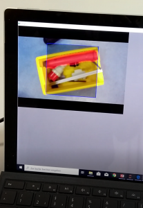
Figure 13 shows a snapshot of the video from the scene (Figure 12) with the predicted mask added. The pixels of the PVC pipe are highlighted with red color.
Conclusion
In this project we created an application to highlight PVC pipes on images from a video. Each image is going through a prediction to create a prediction mask. Each pixel of the mask has two categories: a pixel can be a PVC pipe and a pixel can be no PVC pipe.
To produce masks we trained a U-Net model with training images from the scene. However mask images are needed as well, so they need to be created with a tool. We programmed an ergonomic tool where the user can click on the outline on the PVC pipe of the training image and a polygon is created. An OpenCV function returns the mask image from the polygon. Due to the tediousness of photographing so many training images we augment the images by rotation and flipping. So the number of original training images can multiplied by 72.
The application shows impressively how the PVC pipe is highlighted while the scene has defined items. Note we have perfect light conditions. As soon as new objects are put into the scene, they might be highlighted as well due to insufficient training and wrong prediction. Hence more real training data will be needed, and less training data generated from augmentation. Same is true with the light conditions. So more data is need from different light sources. A very easy thing to do is to augment the data with different contrast and brightness levels.
Ackowledgement
Special thanks to Jan Dieterich who provided the tool to augment the image data. Also special thanks to the University of Applied Science Albstadt-Sigmaringen offering a classroom and appliances to enable this research.