Introduction
The end of each human chromosome consists of a noncoding DNA region, the so called telomere. The telomeric sequence 5′-TTAGGG-3′ is repeated up to several thousand times at every chromosomal end. Each time a cell divides, the DNA of the cell gets replicated. Due to the end replication problem, some telomeric DNA gets lost at each round of replication and a single stranded 3′-overhang is generated. To protect the single stranded 3′-overhang from DNA repair mechanisms, the telomeric DNA is associated with proteins (shelterin complex) and forms a special loop structure (telomere loop and displacement loop). As soon as telomeres reach a critical length and no telomere lengthening mechanisms are available (i.e. telomerase, alternative lengthening of telomeres) the cell stops dividing or cell death is initiated (senescence or apoptosis).
Telomere shortening is an important hallmark of ageing and plays a crucial role in cancer and other diseases like cardiovascular diseases. Furthermore more and more studies arise, which show that behavioral aspects and lifestyle factors can accelerate telomere shortening as well. Therefore, knowing more about telomere biology is essential in ageing research.
There are several methods to measure telomere length. But until now, only the metaphase Q-FISH (Quantitative Fluorescence In Situ Hybridization) method is able to detect and analyze every telomere – even the critically short ones – and assign it to its chromosome. After metaphase preparation the biologist hybridizes telomeres with a fluorescently labeled sequence specific PNA probe and the DNA is stained with DAPI. Afterwards two pictures are taken of each metaphase: one chromosome image and one telomere image.
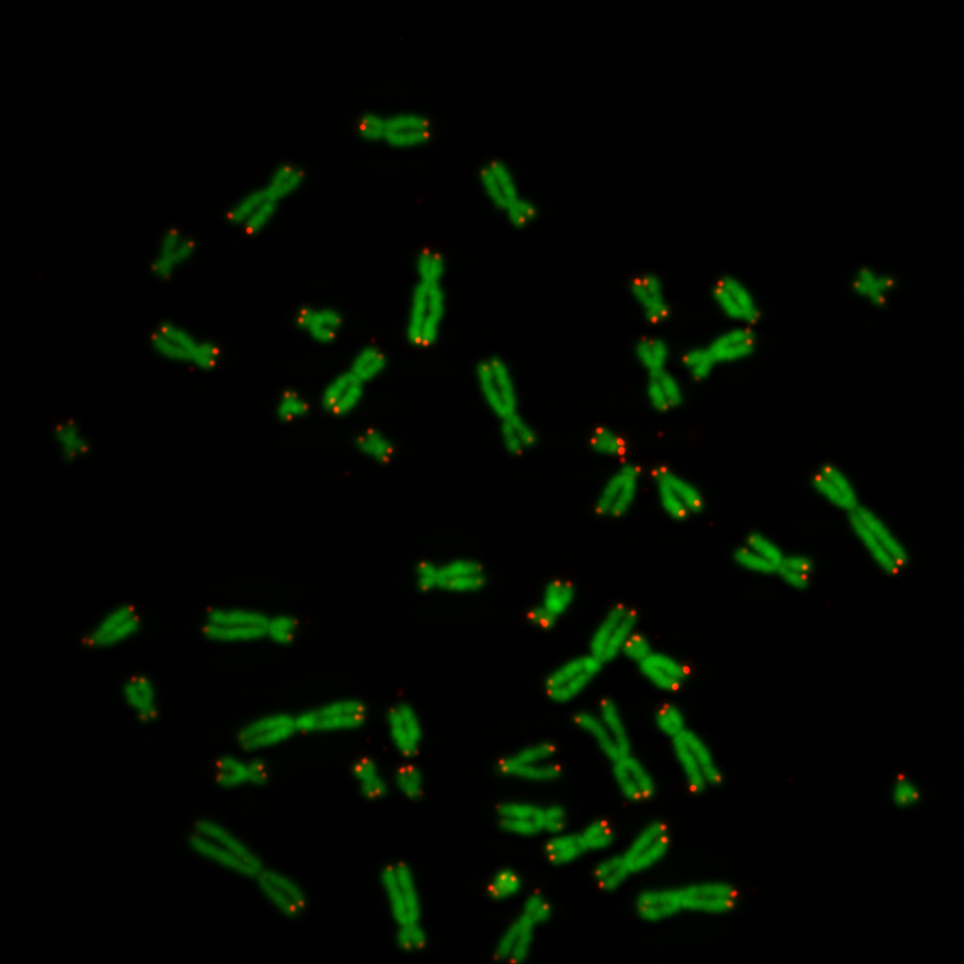
The pixel intensity of telomeres give an indication of the telomere length. So the idea was to segment the regions of telomeres on the telomere image and use them as masks. All pixel intensities behind the masks can be summed to a value which might be an indication of the biological age of the cell. Below a picture of chromosomes and telomeres, Figure 1. The objects in green are the chromosomes and the dots in red are the telomeres. Actually the biologists provide two separate black and white images: a chromosome image and a the telomere image of one cell. In Figure 1 the two images were added to one image for display purpose. The chromosomes image was copied into the green layer and telomere image into the red layer. The pixels of the blue layer were set to 0.
Using U-Nets to create masks
In order to count the pixel intensities on the telomere image, we need to segment the regions on the image to know which pixel is a telomere and which pixel is something else. The pixels can be categorized with three attributes: chromosome, telomere and neither of both. The problem we are facing here is a segmentation problem.
Segmenting images into regions is well known in other applications, such as indicating regions in images showing scenes of traffic. Here the categories of regions can be: street, car, bicycle, tree, building etc. This video shows a nice presentation of an application. The problem to solve is a similar one, however we have less complicated images and we have less categories.
One model which can be used for segmentation is the U-Net. U-Net consists of two parts, a contracting part and a expanding part. At the contracting part, an image is applied to convolutional neural network, followed by relu and maxpooling operations. This is repeated several times, each time the image sizes are reduced, but the number of images increase because a number of filters is applied to them. At the expansion path the images are fed into transposed convolutional neural networks scaling up the images again until one image is left with the same size as the input image. During this convolution process, pixel information from the contracting part is concatenated into the expanding part.
The U-Net used in this project is taken from here. Tobias Sterbak described there his seismic image project using exactly the same neural network model.
#Copyright (c) 2018 Tobias Sterbak
#
#Permission is hereby granted, free of charge, to any person obtaining a copy
#of this software and associated documentation files (the "Software"), to deal
#in the Software without restriction, including without limitation the rights
#to use, copy, modify, merge, publish, distribute, sublicense, and/or sell
#copies of the Software, and to permit persons to whom the Software is
#furnished to do so, subject to the following conditions:
#
#The above copyright notice and this permission notice shall be included in all
#copies or substantial portions of the Software.

def conv2d_block(input_tensor, n_filters, kernel_size=3, batchnorm=True):
    # first layer
    x = Conv2D(filters=n_filters, kernel_size=(kernel_size, kernel_size), kernel_initializer="he_normal",
               padding="same")(input_tensor)
    if batchnorm:
        x = BatchNormalization()(x)
    x = Activation("relu")(x)
    # second layer
    x = Conv2D(filters=n_filters, kernel_size=(kernel_size, kernel_size), kernel_initializer="he_normal",
               padding="same")(x)
    if batchnorm:
        x = BatchNormalization()(x)
    x = Activation("relu")(x)
    return x

def get_unet(input_img, n_filters=16, dropout=0.5, batchnorm=True):
    # contracting path
    c1 = conv2d_block(input_img, n_filters=n_filters*1, kernel_size=3, batchnorm=batchnorm)
    p1 = MaxPooling2D((2, 2)) (c1)
    p1 = Dropout(dropout*0.5)(p1)

    c2 = conv2d_block(p1, n_filters=n_filters*2, kernel_size=3, batchnorm=batchnorm)
    p2 = MaxPooling2D((2, 2)) (c2)
    p2 = Dropout(dropout)(p2)

    c3 = conv2d_block(p2, n_filters=n_filters*4, kernel_size=3, batchnorm=batchnorm)
    p3 = MaxPooling2D((2, 2)) (c3)
    p3 = Dropout(dropout)(p3)

    c4 = conv2d_block(p3, n_filters=n_filters*8, kernel_size=3, batchnorm=batchnorm)
    p4 = MaxPooling2D(pool_size=(2, 2)) (c4)
    p4 = Dropout(dropout)(p4)

    c5 = conv2d_block(p4, n_filters=n_filters*16, kernel_size=3, batchnorm=batchnorm)

    # expansive path
    u6 = Conv2DTranspose(n_filters*8, (3, 3), strides=(2, 2), padding='same') (c5)
    u6 = concatenate([u6, c4])
    u6 = Dropout(dropout)(u6)
    c6 = conv2d_block(u6, n_filters=n_filters*8, kernel_size=3, batchnorm=batchnorm)

    u7 = Conv2DTranspose(n_filters*4, (3, 3), strides=(2, 2), padding='same') (c6)
    u7 = concatenate([u7, c3])
    u7 = Dropout(dropout)(u7)
    c7 = conv2d_block(u7, n_filters=n_filters*4, kernel_size=3, batchnorm=batchnorm)

    u8 = Conv2DTranspose(n_filters*2, (3, 3), strides=(2, 2), padding='same') (c7)
    u8 = concatenate([u8, c2])
    u8 = Dropout(dropout)(u8)
    c8 = conv2d_block(u8, n_filters=n_filters*2, kernel_size=3, batchnorm=batchnorm)

    u9 = Conv2DTranspose(n_filters*1, (3, 3), strides=(2, 2), padding='same') (c8)
    u9 = concatenate([u9, c1], axis=3)
    u9 = Dropout(dropout)(u9)
    c9 = conv2d_block(u9, n_filters=n_filters*1, kernel_size=3, batchnorm=batchnorm)

    outputs = Conv2D(3, (1, 1), activation='sigmoid') (c9)
    model = Model(inputs=[input_img], outputs=[outputs])
    return model
Creating the Training Data Set
Images created by the biologists have the size of about 1900×1300 pixels. Altogether we received about 50 from them. So the pictures are firstly very large and secondly there are not many available. This means, there is too few training data available to train a U-Net.
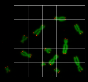
So the idea is, to cut the images into smaller pieces and then to augment the pieces to increase the number of training data. We wrote an application, where the user can draw a rectangle on the chromosome/telomere image with the mouse, and the image pieces for the training data are shown as a grid, see Figure 2. The region of each grid element is copied into an image file. All image files have the size of 80×80.
By doing this, we here able to create about 1200 image files. This is now part of our training data. Since this is still not enough to train a neural network, we augmented the data even further. We will do the augmentation step a little later, because we need to create the mask data first. So the U-Net model needs to be fed with training data and mask data.
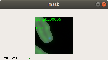
A mask image indicates which pixel belongs to which category on the corresponding training image. Currently we have three categories: Chromosome, telomere and neither of both. We create the masks with second application, which displays the training image and the user can adjust the contrast and the threshold using the mouse and keyboard. Figure 3 shows how the output looks like after the user adjusts the threshold level of a training image. Additional filters adjust the contrast and the brightness. The application saves the mask image and to precede with the next training image. Figure 3 shows the complete chromosome/telomere image and an overlayed mask. The chromosome image, the telomere image and the mask image where added here together. However, the application solely saves the mask image.
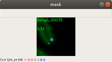
Below an example for creating a telomere mask from the same training image. Here the same features of the applications can be used for threshold, contrast and brightness adjustment. Figure 4 shows the combined chromosome image, telomere image and mask image. This is for display purpose. The application saves only the telomere mask.
The following Figure 5 shows five training data images. The chromosome images and the telomere images are actually stored separately. For display purpose, we added them together Figure 5. However, for training purpose of the neural network, we also combine the chromosome and telomere images to three layered RGB images. The chromosome image is copied to the green layer and the telomere picture to the red layer. The pixels values of the blue layer are set to 0.
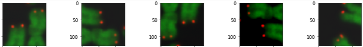
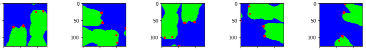
Figure 6 shows the mask images created by the user with the second application we programmed from the images of Figure 5. Again each of the images are actually two images, which are added together for display purpose. However for training, we use exactly these combined images. Since we have three categories, chromosome, telomere or neither of both, we can use three colors to display this information. Green pixel are chromosomes, red pixels are telomeres and blue pixels are neither of both.
We created just 1200 training images from the original pictures. So we created 1200 mask images with the application we provided. We mentioned, that the number of images is to low for running a training process on a neural network. In order to have enough data, we augment the data. Augmentation is simply done by rotation of each training image and each mask image. Also, the images are flipped and rotated again. All images were stored, so we increased the training set from 1200 to 9600 images. At each rotation step, we applied a random change of contrast and brightness to each training image to get some variance within the image. We assume that this has a beneficial effect for prediction. The mask images were rotated and flipped exactly the same way as the training images.
Training of the U-Net
The model was compiled with the categorical cross entropy loss function which supports to exclusively distinguish between categories, which are chromosome, telomere and neither of both pixels. We use sigmoid as an activation function (see U-Net Model above), which delivers a number between 0 and 1 for each pixel as an outcome. One could argue that softmax would be a better activation function, but sigmoid delivered just good results. Below the code, which compiles the U-Model.
input_img = Input((im_height, im_width, 3), name='img')
model = get_unet(input_img, n_filters=16, dropout=0.05, batchnorm=True)
model.compile(optimizer=Adam(), loss="categorical_crossentropy", metrics=["accuracy"])
Before starting the training process, the training data and the mask data are normalized. On each training image the average function and the standard deviation function was applied. The pixels of the mask images were set to 1 or to 0 depending on the original value. This can be done by dividing the pixel value with 255, see code below.
# normalize training data
train_data -= train_data.mean()
train_data /= train_data.std()
#normalize mask data
train_mask //= 255
A callback function was used to automatically save a snapshot of the model, if the training process shows an improvement after an epoch. The code below shows the fit function with train_data containing the normalized training images and the train_mask containing the normalized mask images. In a similar way this is done with the validation data. In this case about 20% of the training and mask data were used for validation.
callbacks = [
    EarlyStopping(patience=10, verbose=1),
    ReduceLROnPlateau(factor=0.1, patience=3, min_lr=0.00001, verbose=1),
    ModelCheckpoint('modelbio.h5', verbose=1, save_best_only=True, save_weights_only=True)
]
results = model.fit(train_data, train_mask, batch_size=32, epochs=20, callbacks=callbacks, validation_data=(valid_data, valid_mask))
After about 17 epochs, there has not been shown any training improvement and the training was stopped. The accuracy was about 0.993 and the validation accuracy 0.9907. The loss was 0.0157 and the validation loss 0.0236. The results of the loss functions show a light overfitting. Using a NVIDIA 2070 GPU, the training took about 5 minutes. After training the model was saved for the final QFISH application.
Determining Telomere Lengths
The goal of the project is to determine the lengths of all telomeres on images created by the biologist. The biologist actually provides two black and white images, the chromosome image and the telomere image, both are exactly aligned to each other. As mentioned above, for training and predicting purpose, we add these two images to one combined image. So the chromosome image is copied into the green layer, and the telemore image into the red layer. The pixels of the blue layer are set to 0.
The user of the QFISH application is selecting a region on the combined image, and grid images with the size of 80×80 are extracted from the region, see also Figure 2. These grid images are normalized and then fed into the trained model which predicts masks from them. The code below shows how the grid images (predict_data) are normalized and how the predicted masks (prediction_masks) are generated from prediction.
predict_data -= predict_data.mean()
predict_data /= predict_data.std()
prediction_masks = model.predict(predict_data, batch_size=50, verbose=1)
The predicted masks from the prediction output are assembled together to a picture with the size of the previously selected region. During the training process of the U-Net, we used the sigmoid activation function on each pixel, whose value indicates if the pixel is a chromosome, a telomere or neither of both. So the QFISH application compares at each pixel position of the assembled picture the values on each layer. The highest value of each layer is taken and this value is replaced by the maximum value which is 255. The other two layer values of that pixel are set to 0. Figure 7 shows the output. It can be seen that the green pixels mark the chromosomes, and the red pixels mark the telomeres. The pixels which are neither of both are shown in blue:
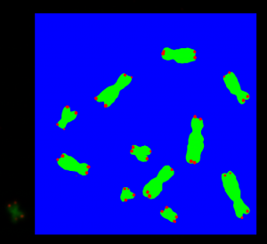
The layers and its pixel values of the assembled picture indicate now if a pixel is a chromosome, a telomere or neither of both. This is also shown by the colors of each pixel, see Figure 7.
The blue layer of the assembled picture contain information, that the pixel is neither chromosome nor telomere. We use this blue layer to create contours with the tool OpenCV. Figure 8 shows eleven chromosome/telomere contours. Ideally it should be 46 contours, because this is the number of chromosomes for each cell, but we simplify this for explanation purpose.
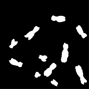
However in some cases the chromosomes lie too close to each other, and other cases there is some noise on the original pictures provided by the biologist. The noise is filtered out by removing all contours which have areas below a threshold.
To obtain the telomere pixel intensities, we firstly create a new picture from one of the contours (Figure 8) which is now a single chromosome mask. A second new picture is created from the contours of the telemore layer (red layer) of the assembled picture. A third new picture is created by using the image AND operation on the single chromosome mask (first new picture) , the contours of the telomere layer (second new picture) and the original telomere image provided by the biologist. After the AND operation we have the pixels of the telomeres of one chromosome. The QFISH application just adds the pixel values of the third new picture which results to the telomere pixel intensities of one chromosome.
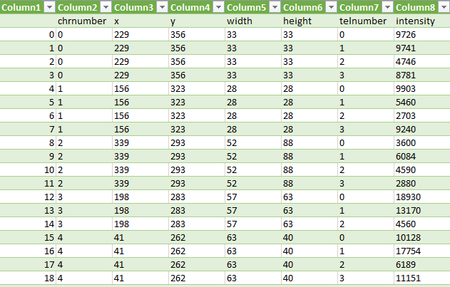
These three steps are repeated for each chromosome contour (Figure 8) and we receive the intensities of the telomeres. The values are then written into a comma separate value file, see Figure 9.
Conclusion
In this post it was shown how telomere intensities can be extracted from original chromosome and telomere images. We use a neuronal network, which was trained previously with data provided by the biologists, to obtain masks of chromosomes and telomeres. The contours of the masks were used to mask out the needed telomere regions from the original images. Pixel value of the telomeres we added up to receive an indication of the telomere length. All information is stored in a csv file.
Acknowledgement
Special thanks to the Hochschule Albstadt-Sigmaringen which financed this research under the program Fit4Research. Also thanks to the Life Science Faculty, which provided the chromosome and telemore pictures.