In a previous blog we documented methods and code for recognizing fruits with a neural network on a raspberry pi. This time we want to go one step further and describe the method and code to create heatmaps for fruit images. The method we use here is called Gradient-weighted Class Activation Mapping (Grad-CAM). A heatmap is telling us which pixel of an fruit image leads to the neural network’s decision to assign the input image to a specific class.
We believe that heatmaps are a very useful information especially during the validation after a neural network is trained. We want to know, if the neural networks is really making the right decision upon the given information (such as a fruit image). A good example is the classification of wolf and husky dog images made once by researchers (“Why Should I Trust You?”, See Reference). The researchers had actually pretty good results, until somebody figured out, that most wolf images were taken in a snowy environment, while the husky images were not. The neural network mostly associated a snowy environment with a wolf. The husky dog was therefore classified as wolf, when the image was taken with snow in the background.
For a deeper neural network validation, we can use heatmaps to see how the classification decision was made. Below we will show you how we generate heatmaps from fruit images. The Keras website helped us a lot to write our code, see also Reference.
The Setup
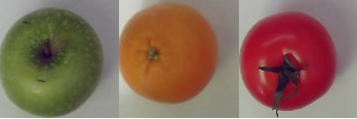
We use three different classes of images: Apfel (appel) images, orange images and tomate (tomato) images, see Figure 1. The list classes, see code below, contains strings describing the classes. We filled in the training, validation and test directories with fruit images, similar to those in Figure 1. Each class of fruit images went into its own directory named Apfel, Orange and Tomate.
In the code below we use the paths traindir, a validdir and a testdir. The weights and the structure of the neural network model (modelsaved and modeljson) is saved into the model directory .
The classes Apfel, Orange and Tomate are associated to numbers with the python classnum dictionary. The variable dim defines the size of the images.
basepath = "/home/....../Session1"
traindir = os.path.join(basepath, "pics" , "train")
validdir = os.path.join(basepath, "pics" , 'valid')
testdir = os.path.join(basepath, "pics" , 'test')
model_path = os.path.join(basepath, 'models')

classes = ["Apfel","Orange","Tomate"]
classnum = {"Apfel":0, "Orange":1, "Tomate":2}

net = 'convnet'

now = datetime.datetime.now()

modelweightname = f"model_{net}_{now.year}-{now.month}-{now.day}_callback.h5"
modelsaved = f"model_{net}.h5"
modeljson = f"model_{net}.json"


dim = (100,100, 3)
The Model
The following code shows the convolutional neural network (CNN) code in Keras. We have four convolutional layers and two dense layers. The last dense layer has three neurons. The output of one neuron indicates if an image is predicted as an apple, an orange or a tomato. Since the output is exclusive (an apple cannot be a tomato), we use the softmax activation function for the last layer.
def create_conv_net():
    model = Sequential()
    model.add(Conv2D(32, (3, 3), activation='relu', kernel_initializer='he_uniform', padding='same', input_shape=(dim[0], dim[1], 3)))
    model.add(BatchNormalization())
    model.add(MaxPooling2D((2, 2)))
    model.add(Conv2D(32, (3, 3), activation='relu', kernel_initializer='he_uniform', padding='same'))
    model.add(BatchNormalization())
    model.add(MaxPooling2D((2, 2)))
    model.add(Conv2D(64, (3, 3), activation='relu', kernel_initializer='he_uniform', padding='same'))
    model.add(BatchNormalization())
    model.add(MaxPooling2D((2, 2)))
    model.add(Conv2D(128, (3, 3), activation='relu', kernel_initializer='he_uniform', padding='same'))
    model.add(BatchNormalization())
    model.add(MaxPooling2D((2, 2)))
    model.add(Flatten())
    model.add(Dense(128, activation='relu', kernel_initializer='he_uniform'))
    model.add(Dense(len(classes), activation='softmax'))
    #opt = Adam(lr=1e-3, decay=1e-3 / 200)
    return model
The function create_conv_net creates the model. It is compiled with categorical_crossentropy loss function, see code below.
model = create_conv_net()
model.compile(Adam(lr=.00001), loss="categorical_crossentropy", metrics=['accuracy'])
The focus here is to describe the Grad-Cam method, and not the training of the model. Therefore we leave out the specifics on training. More details on training can be found here. The code below loads in (Keras method load_weights) a previously prepared model checkpoint and shows with the summary method the structure of the model. This is a useful information, because we have to look for the last convolutional layer. It is needed later.
model.load_weights(os.path.join(model_path,"model_convnet_2021-7-1_callback.h5"))
model.summary()
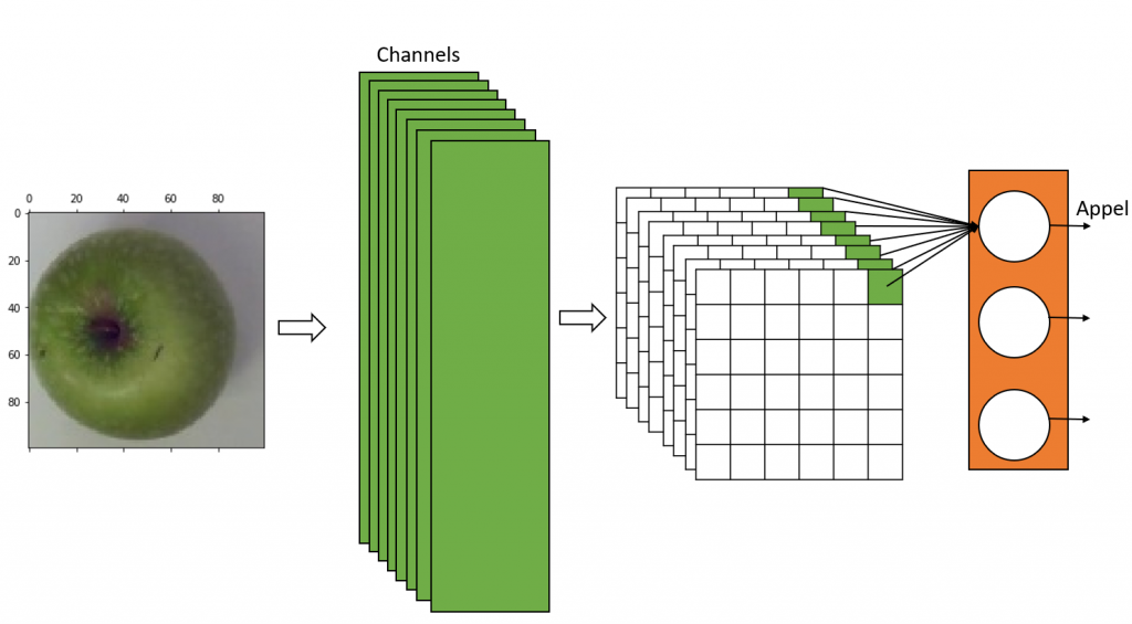
Now we have to create a new model with two outputs layers. In Figure 2 you see a simplified representation of the CNN we use. The last layer (color orange) represents the dense layer. The last CNN layer is in color green. Due to the filters of the CNN layer we have numerous channels. The Grad-CAM method requires the outputs of the channels. So we need to create a new model, based on the one above, which outputs both, the images of the results of the channels from the last CNN layer and the classification decision from the dense layer.
The code below iterates through the layers of CNN model in reverse order and finds the last batch_normalization layer. We modeled the neural network in a way that each CNN layer is followed by the batch_normalization layer, so we pick the batch_normalization layer as an output. The code produces a new model gradModel with model‘s input; and model‘s last CNN layer (actually last batch_nomalization layer) and last dense layer as outputs.
gradModel = None

for layer in reversed(model.layers):
    if "batch_normalization" in layer.name:
        print(layer.name)
        gradModel = Model(inputs=model.inputs, outputs=[model.get_layer(layer.name).output, model.output])
        break
The Grad-CAM method
The function getGrad below is executing the model gradModel with an image given as a parameter img. It returns the results (conv, predictions) of the last CNN layer (actually batch_normalization) and the last dense layer. We are now interested in the gradients of the images returned from the last CNN layer with respect to the loss of a specific class. The dictionary classnum (defined above) outputs a class number and addresses the loss inside predictions, see command below.
loss = predictions[:, classnum[classname]]
The gradients of the last CNN layer with respect to the loss of a specific class are calculated with tape‘s gradient method. The function getGrad returns the input image, the output of the last CNN layer (conv) and the gradients of the last CNN layer.
def getGrad(img, classname):

    testpics = np.array([img], dtype=np.float32)

    with tf.GradientTape() as tape:

        conv, predictions =  gradModel(tf.cast(testpics, tf.float32))

        loss = predictions[:, classnum[classname]]

    grads = tape.gradient(loss, conv)

    return img, conv, grads
The function getHeatMap below creates a heatmap from the output of the image’s last CNN layer and its gradients. Inside getHeadMap, the Tensorflow method reduce_mean takes the mean values (pooled_grads) of grads. The mean value is an indication of how important the output of a channel from the last CNN layer is. The function multiplies its mean values with the corresponding CNN layer outputs (convpic) and sums up the output into heatmap. Since we want to have an image to look at, the function getHeatMap is rectifying, normalizing and resizing the heatmap before it is returning it.
def getHeatMap(conv, grads):
    pooled_grads = tf.reduce_mean(grads, axis=(0, 1, 2))
    convpic = conv[0]
    heatmap = convpic @ pooled_grads[..., tf.newaxis]
    heatmapsq = tf.squeeze(heatmap)
    heatmapnorm = tf.maximum(heatmapsq, 0) / tf.math.reduce_max(heatmapsq)
    heatmapnp = heatmapnorm.numpy()
    heatmapresized = cv2.resize(heatmapnp, (dim[0], dim[1]), interpolation = cv2.INTER_AREA)*255
    heatmapresized = heatmapresized.astype("uint8")
    ret = np.zeros((dim[0], dim[1]), 'uint8')
    ret = heatmapresized.copy()
    return ret
Testing the images
The apple, orange and tomato images are stored in separate directories. So the function testgrads, see code below, loads in the images from the test directory into the pics0, pics1 and pics2 lists. They are then added together into pics list.
The function testgrads normalizes the list of images and predicts its classifications (variable predictions). The function testgrads calls the getGrad function and the getHeatMap function to receive a heatmap for each image. Numpy’s argmax methods outputs a number which indicates if the image is an apple, an orange or a tomato and moves the result into pos. Finally the heatmap, which is a grayscale image, is converted into a color image (apple images are converted in green color, orange images into blue color and tomato images into red color). The function testgrads is then returning a list of colored heatmaps for each image.
def testgrads(picdir):

    pics0 = [os.path.join(picdir, classes[0], f) for f in os.listdir(os.path.join(picdir, classes[0]))]
    pics1 = [os.path.join(picdir, classes[1], f) for f in os.listdir(os.path.join(picdir, classes[1]))]
    pics2 = [os.path.join(picdir, classes[2], f) for f in os.listdir(os.path.join(picdir, classes[2]))]

    pics = pics0 + pics1 + pics2

    imagelist = []

    for pic in pics:
        img = np.zeros((dim[0], dim[1],3), 'uint8')
        img = cv2.resize(cv2.imread(pic,cv2.IMREAD_COLOR ), (dim[0], dim[1]), interpolation = cv2.INTER_AREA)
        imagelist.append(img)

    train_data = np.array(imagelist, dtype=np.float32)

    train_data -= train_data.mean()
    train_data /= train_data.std()

    predictions = model.predict(train_data)

    heatmaps = []

    for i in range(len(train_data)):
        heatmapc = np.zeros((dim[0], dim[1],3), 'uint8')
        pos = np.argmax(predictions[i])
        img, conv, grads = getGrad(train_data[i], classes[pos])
        heatmap =  getHeatMap(conv, grads)

        if pos == 0:
            posadj = 1
        elif pos == 1:
            posadj = 0
        elif pos == 2:
            posadj = 2

        heatmapc[:,:,posadj] = heatmap[:,:]

        heatmaps.append(heatmapc)


    return imagelist, heatmaps
Below the code which calls the function testgrads. The parameter testdir is the path of the test images.
imagelist, heatlist = testgrads(testdir)
Result
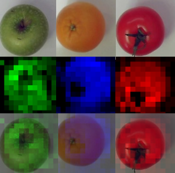
In Figure 3 you find three images (apple, orange and tomato) passed through the testgrads function, see top row. In the middle row, you find the outputs of the testgrads function. These are the visualized heatmaps. The bottom row of Figure 3 are images which were merged with OpenCV’s weighted method. So the heatmap pixels indicate, which group of pixels of the original image led to the prediction decision. You see that the black heatmaps pixels indicate that the background pixels do not lead to any decision. The same is true for the fruit stems.
References
Keras: https://keras.io/examples/vision/grad_cam/
pyimagesearch: https://www.pyimagesearch.com/2020/03/09/grad-cam-visualize-class-activation-maps-with-keras-tensorflow-and-deep-learning/
Why should I trust you: https://arxiv.org/pdf/1602.04938.pdf
Fruit Recognition: https://www3.hs-albsig.de/wordpress/point2pointmotion/2020/03/26/fruit-recognition-on-a-raspberry-pi/