In a previous blog we documented methods and code for recognizing fruits with a neural network on a raspberry pi. This time we want to go one step further and describe the method and code to create heatmaps for fruit images. The method we use here is called Gradient-weighted Class Activation Mapping (Grad-CAM). A heatmap is telling us which pixel of an fruit image leads to the neural network’s decision to assign the input image to a specific class.
We believe that heatmaps are a very useful information especially during the validation after a neural network is trained. We want to know, if the neural networks is really making the right decision upon the given information (such as a fruit image). A good example is the classification of wolf and husky dog images made once by researchers (“Why Should I Trust You?”, See Reference). The researchers had actually pretty good results, until somebody figured out, that most wolf images were taken in a snowy environment, while the husky images were not. The neural network mostly associated a snowy environment with a wolf. The husky dog was therefore classified as wolf, when the image was taken with snow in the background.
For a deeper neural network validation, we can use heatmaps to see how the classification decision was made. Below we will show you how we generate heatmaps from fruit images. The Keras website helped us a lot to write our code, see also Reference.
The Setup
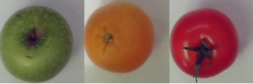
We use three different classes of images: Apfel (appel) images, orange images and tomate (tomato) images, see Figure 1. The list classes, see code below, contains strings describing the classes. We filled in the training, validation and test directories with fruit images, similar to those in Figure 1. Each class of fruit images went into its own directory named Apfel, Orange and Tomate.
Figure 1: Images of an appel, an orange and a tomato
In the code below we use the paths traindir, a validdir and a testdir. The weights and the structure of the neural network model (modelsaved and modeljson) is saved into the model directory .
The classes Apfel, Orange and Tomate are associated to numbers with the python classnum dictionary. The variable dim defines the size of the images.
The following code shows the convolutional neural network (CNN) code in Keras. We have four convolutional layers and two dense layers. The last dense layer has three neurons. The output of one neuron indicates if an image is predicted as an apple, an orange or a tomato. Since the output is exclusive (an apple cannot be a tomato), we use the softmax activation function for the last layer.
The function create_conv_net creates the model. It is compiled with categorical_crossentropy loss function, see code below.
model = create_conv_net()
model.compile(Adam(lr=.00001), loss="categorical_crossentropy", metrics=['accuracy'])
The focus here is to describe the Grad-Cam method, and not the training of the model. Therefore we leave out the specifics on training. More details on training can be found here. The code below loads in (Keras method load_weights) a previously prepared model checkpoint and shows with the summary method the structure of the model. This is a useful information, because we have to look for the last convolutional layer. It is needed later.
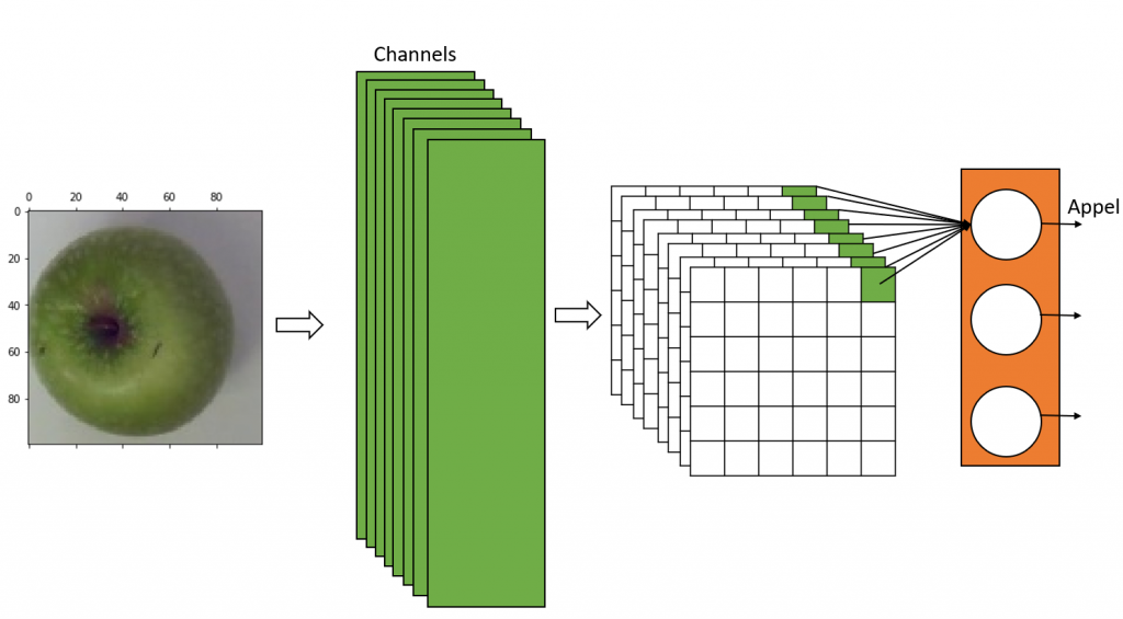
Now we have to create a new model with two outputs layers. In Figure 2 you see a simplified representation of the CNN we use. The last layer (color orange) represents the dense layer. The last CNN layer is in color green. Due to the filters of the CNN layer we have numerous channels. The Grad-CAM method requires the outputs of the channels. So we need to create a new model, based on the one above, which outputs both, the images of the results of the channels from the last CNN layer and the classification decision from the dense layer.
Figure 2: Simplified CNN
The code below iterates through the layers of CNN model in reverse order and finds the last batch_normalization layer. We modeled the neural network in a way that each CNN layer is followed by the batch_normalization layer, so we pick the batch_normalization layer as an output. The code produces a new model gradModel with model‘s input; and model‘s last CNN layer (actually last batch_nomalization layer) and last dense layer as outputs.
gradModel = None

for layer in reversed(model.layers):
    if "batch_normalization" in layer.name:
        print(layer.name)
        gradModel = Model(inputs=model.inputs, outputs=[model.get_layer(layer.name).output, model.output])
        break
The Grad-CAM method
The function getGrad below is executing the model gradModel with an image given as a parameter img. It returns the results (conv, predictions) of the last CNN layer (actually batch_normalization) and the last dense layer. We are now interested in the gradients of the images returned from the last CNN layer with respect to the loss of a specific class. The dictionary classnum (defined above) outputs a class number and addresses the loss inside predictions, see command below.
loss = predictions[:, classnum[classname]]
The gradients of the last CNN layer with respect to the loss of a specific class are calculated with tape‘s gradient method. The function getGrad returns the input image, the output of the last CNN layer (conv) and the gradients of the last CNN layer.
def getGrad(img, classname):

    testpics = np.array([img], dtype=np.float32)

    with tf.GradientTape() as tape:

        conv, predictions =  gradModel(tf.cast(testpics, tf.float32))

        loss = predictions[:, classnum[classname]]

    grads = tape.gradient(loss, conv)

    return img, conv, grads
The function getHeatMap below creates a heatmap from the output of the image’s last CNN layer and its gradients. Inside getHeadMap, the Tensorflow method reduce_mean takes the mean values (pooled_grads) of grads. The mean value is an indication of how important the output of a channel from the last CNN layer is. The function multiplies its mean values with the corresponding CNN layer outputs (convpic) and sums up the output into heatmap. Since we want to have an image to look at, the function getHeatMap is rectifying, normalizing and resizing the heatmap before it is returning it.
The apple, orange and tomato images are stored in separate directories. So the function testgrads, see code below, loads in the images from the test directory into the pics0, pics1 and pics2 lists. They are then added together into pics list.
The function testgrads normalizes the list of images and predicts its classifications (variable predictions). The function testgrads calls the getGrad function and the getHeatMap function to receive a heatmap for each image. Numpy’s argmax methods outputs a number which indicates if the image is an apple, an orange or a tomato and moves the result into pos. Finally the heatmap, which is a grayscale image, is converted into a color image (apple images are converted in green color, orange images into blue color and tomato images into red color). The function testgrads is then returning a list of colored heatmaps for each image.
def testgrads(picdir):

    pics0 = [os.path.join(picdir, classes[0], f) for f in os.listdir(os.path.join(picdir, classes[0]))]
    pics1 = [os.path.join(picdir, classes[1], f) for f in os.listdir(os.path.join(picdir, classes[1]))]
    pics2 = [os.path.join(picdir, classes[2], f) for f in os.listdir(os.path.join(picdir, classes[2]))]

    pics = pics0 + pics1 + pics2

    imagelist = []

    for pic in pics:
        img = np.zeros((dim[0], dim[1],3), 'uint8')
        img = cv2.resize(cv2.imread(pic,cv2.IMREAD_COLOR ), (dim[0], dim[1]), interpolation = cv2.INTER_AREA)
        imagelist.append(img)

    train_data = np.array(imagelist, dtype=np.float32)

    train_data -= train_data.mean()
    train_data /= train_data.std()

    predictions = model.predict(train_data)

    heatmaps = []

    for i in range(len(train_data)):
        heatmapc = np.zeros((dim[0], dim[1],3), 'uint8')
        pos = np.argmax(predictions[i])
        img, conv, grads = getGrad(train_data[i], classes[pos])
        heatmap =  getHeatMap(conv, grads)

        if pos == 0:
            posadj = 1
        elif pos == 1:
            posadj = 0
        elif pos == 2:
            posadj = 2

        heatmapc[:,:,posadj] = heatmap[:,:]

        heatmaps.append(heatmapc)


    return imagelist, heatmaps
Below the code which calls the function testgrads. The parameter testdir is the path of the test images.
imagelist, heatlist = testgrads(testdir)
Result
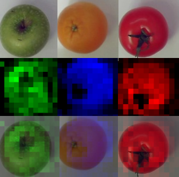
In Figure 3 you find three images (apple, orange and tomato) passed through the testgrads function, see top row. In the middle row, you find the outputs of the testgrads function. These are the visualized heatmaps. The bottom row of Figure 3 are images which were merged with OpenCV’s weighted method. So the heatmap pixels indicate, which group of pixels of the original image led to the prediction decision. You see that the black heatmaps pixels indicate that the background pixels do not lead to any decision. The same is true for the fruit stems.
For the summer semester 2020 we offered an elective class called Design Cyber Physical Systems. This time only few students enrolled into the class. The advantage of having small classes is that we can focus on a certain topic without loosing the overview during project execution. The class starts with a brain storming session to choose a topic to be worked on during the semester. There are only a few constraints which we ask to apply. The topic must have something to do with image processing, neural networks and deep learning. The students came up with five ideas and presented them to the instructor. The instructor commented on the ideas and evaluated them. Finally the students chose one of the idea to work on until the end of the semester.
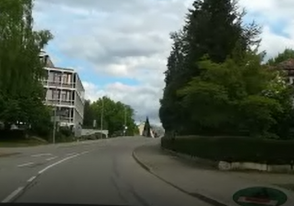
This time the students chose to process street scenes taken from videos while driving a car. A street scene can be seen in Figure 1. The videos were taken in driving direction through the front window of a car. The assignment the students have given to themselves is to extract street, street marking, traffic signs, and cars on the video images. This kind of problem is called semantic segmentation, which has been solved in a similar fashion as in the previous post. Therefore many functions in this post and in the last post are pretty similar.
Figure 1: Street scene
Creating Training Data
The students took about ten videos while driving a car to create the training data. Since videos are just a sequence of images, they selected randomly around 250 images from the videos. Above we mentioned that we wanted to extract street, street marking, traffic signs and cars. These are four categories. There is another one, which is neither of those (or the background category). This makes it five categories. Below you find code of python dictionaries. The first is the dictionary classes which assigns text to the category numbers (such as the number 1 is assigned to Strasse (Street in English). The dictionary categories assigns it the way around. Finally the dictionary colors assigns a color to each category number.
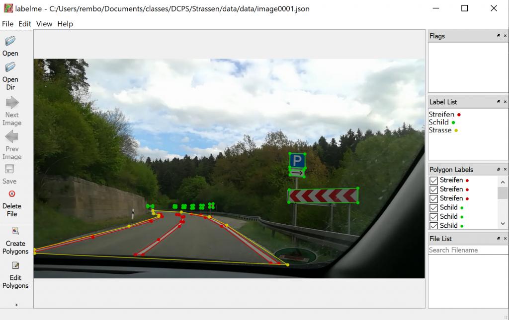
To create training data we decided to use the tool labelme, which is described here. You can load images into the tool, and mark regions by drawing polygons around them, see Figure 2. The regions can be categorized with a names which are the same as from the python dictionary categories, see code above. You can save the polygons, its categories and the image itself to a json file. Now it is very easy to parse the json file with a python parser.
Figure 2: Tool labelme
The image itself is stored in the json file in a base-64 representation. Here python has tools as well, to parse out the image. Videos generally do not store square images, so we need to convert them into a square image, which is better for training the neural network. We have written the following two functions to fulfill this task: makesquare2 and makesquare3. The difference of these functions is, that the first handles grayscale images and the second RGB images. Both functions just omits evenly the left and the right portion of the original video image to create a square image.
Below you see two functions createMasks and createMasksAugmented. We need the functions to create training data from the json files, such as original images and mask images. Both functions have been described in the post before. Therefore we dig only into the differences.
In both functions you find a special handling for the category Strasse (Street in English). You can find it below the code snippet:
classes[shape[‘label’]] != classes[‘Strasse’]
Regions in the images, which are marked as Strasse (Street in English) can share the same region as Streifen (Street Marking in English) or Auto (Car in English). We do not want that street regions overrule the street marking or car regions, otherwise the street marking or the cars will disappear. For this we create first a separate mask mask_strasse. All other category masks are substracted from mask_strasse, and then mask_strasse is added to the finalmask. Again, we just want to make sure that the street marking mask and the other masks are not overwritten by the street mask.
def createMasks(sourcejsonsdir, destimagesdir, destmasksdir):

    assocf = open(os.path.join(path,"assoc_orig.txt"), "w")
    count = 0
    directory = sourcejsonsdir
    for filename in os.listdir(directory):
        if filename.endswith(".json"):
            print("{}:{}".format(count,os.path.join(directory, filename)))

            f = open(os.path.join(directory, filename))
            data = json.load(f)
            img_arr = data['imageData']
            imgdata = base64.b64decode(img_arr)

            img = cv2.imdecode(np.frombuffer(imgdata, dtype=np.uint8), flags=cv2.IMREAD_COLOR)

            assert (img.shape[0] > dim[0])
            assert (img.shape[1] > dim[1])

            finalmask = np.zeros((img.shape[0], img.shape[1]), 'uint8')

            masks=[]
            masks_strassen=[]
            mask_strasse = np.zeros((img.shape[0], img.shape[1]), 'uint8')

            for shape in data['shapes']:
                assert(shape['label'] in classes)

                vertices = np.array([[point[1],point[0]] for point in shape['points']])
                vertices = vertices.astype(int)

                rr, cc = polygon(vertices[:,0], vertices[:,1], img.shape)
                mask_orig = np.zeros((img.shape[0], img.shape[1]), 'uint8')

                mask_orig[rr,cc] = classes[shape['label']]
                if classes[shape['label']] != classes['Strasse']:
                    masks.append(mask_orig)
                else:
                    masks_strassen.append(mask_orig)

            for m in masks_strassen:
                mask_strasse += m

            for m in masks:
                _,mthresh = cv2.threshold(m,0,255,cv2.THRESH_BINARY_INV)
                finalmask = cv2.bitwise_and(finalmask,finalmask,mask = mthresh)
                finalmask += m

            _,mthresh = cv2.threshold(finalmask,0,255,cv2.THRESH_BINARY_INV)
            mask_strasse = cv2.bitwise_and(mask_strasse,mask_strasse, mask = mthresh)
            finalmask += mask_strasse

            img = makesquare3(img)
            finalmask = makesquare2(finalmask)

            img_resized = cv2.resize(img, dim, interpolation = cv2.INTER_NEAREST)
            finalmask_resized = cv2.resize(finalmask, dim, interpolation = cv2.INTER_NEAREST)

            filepure,extension = splitext(filename)

            cv2.imwrite(os.path.join(destimagesdir, "{}o.png".format(filepure)), img_resized)
            cv2.imwrite(os.path.join(destmasksdir, "{}o.png".format(filepure)), finalmask_resized)

            assocf.write("{:05d}o:{}\n".format(count,filename))
            assocf.flush()
            count += 1

        else:
            continue
    f.close()
In createMask you find the usage of makesquare3 and makesquare2, since the video images are not square. However we prefer to use square image for neural network training.
The function createMasksAugmented above does basically the same thing as createMasks, but the image is randomly zoomed and rotated. Also the brightness and contrast is randomly adjusted. The purpose is to create more varieties of images from the original image for regularization.
The original images and mask images for neural network training can be generated by calling the functions below. In the directory fullpathjson you find the source json files. The parameters fullpathimages and fullpathmasks are the directory names for the destination.
Since we labeled 250 video images and stored them to json files, the functions below create altogether 1000 original and mask images. The function createMasksAugmented can be called even more often for more data.
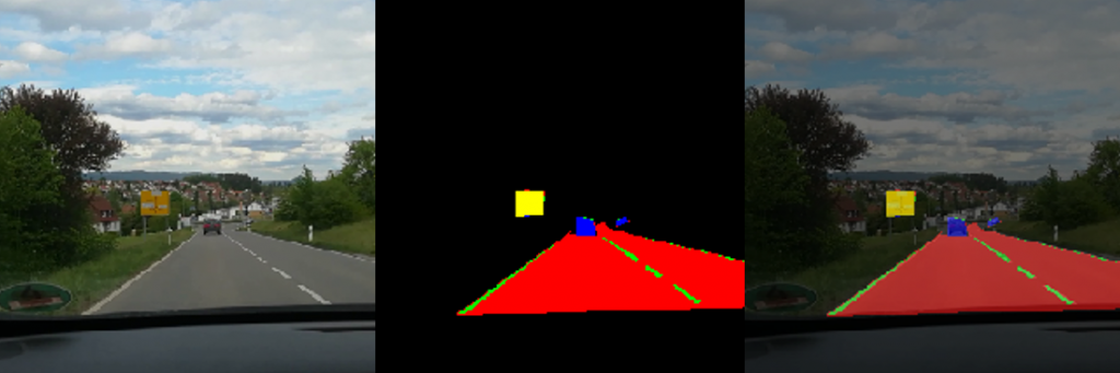
In Figure 3 below you find one result of the applied createMasks function. Left, there is an original image. In the middle there is the corresponding mask image. On the right there is the overlaid image. The region of the traffic sign is marked yellow, the street has color red, the street marking is in green and finally the car has a blue color.
Figure 3: Original Image, mask image and overlaid image
Training the model
We used different kinds of UNET models and compared the results from them. The UNET model from the previous post had mediocre results. For this reason we switched to an UNET model from a different author. It can be found here. The library keras_segmentation gave us much better predictions. However we do not have so much control over the model itself, for this was the reason we created our own UNET model, but we were inspired by keras_segmentation.
Above we already stated that we have five categories. Each category gets a number and a color assigned. The assignment can be seen in the python dictionary below.
The UNET model we created is shown in the code below. It consists of a contracting and an expanding path. In the expanding path we have five convolution operations, followed by batch normalizations, relu-activations and maxpoolings. In between we also use dropouts for regularization. The results of these operations are saved into variables (c0, c1, c2, c3, c4). In the expanding path we implemented the upsampling operations and concatenate their outputs with the variables (c0, c1, c2, c3, c4) from the contracting path. Finally the code performs a softmax operation.
In general the concatenation of the outputs with the variables show benefits during training. Gradients of upper layers often vanish during the backpropagation operation. Concatenation is the method to prevent this behavior. However if this is really the case here has not been proofed.
def my_unet(classes):

    dropout = 0.4
    input_img = Input(shape=(dim[0], dim[1], 3))

    #contracting path
    x = (ZeroPadding2D((1, 1)))(input_img)
    x = (Conv2D(64, (3, 3), padding='valid'))(x)
    x = (BatchNormalization())(x)
    x = (Activation('relu'))(x)
    x = (MaxPooling2D((2, 2)))(x)
    c0 = Dropout(dropout)(x)

    x = (ZeroPadding2D((1, 1)))(c0)
    x = (Conv2D(128, (3, 3),padding='valid'))(x)
    x = (BatchNormalization())(x)
    x = (Activation('relu'))(x)
    x = (MaxPooling2D((2, 2)))(x)
    c1 = Dropout(dropout)(x)

    x = (ZeroPadding2D((1, 1)))(c1)
    x = (Conv2D(256, (3, 3), padding='valid'))(x)
    x = (BatchNormalization())(x)
    x = (Activation('relu'))(x)
    x = (MaxPooling2D((2, 2)))(x)
    c2 = Dropout(dropout)(x)

    x = (ZeroPadding2D((1, 1)))(c2)
    x = (Conv2D(256, (3, 3), padding='valid'))(x)
    x = (BatchNormalization())(x)
    x = (Activation('relu'))(x)
    x = (MaxPooling2D((2, 2)))(x)
    c3 = Dropout(dropout)(x)

    x = (ZeroPadding2D((1, 1)))(c3)
    x = (Conv2D(512, (3, 3), padding='valid'))(x)
    c4 = (BatchNormalization())(x)

    #expanding path
    x = (UpSampling2D((2, 2)))(c4)
    x = (concatenate([x, c2], axis=-1))
    x = Dropout(dropout)(x)
    x = (ZeroPadding2D((1, 1)))(x)
    x = (Conv2D(256, (3, 3), padding='valid', activation='relu'))(x)
    e4 = (BatchNormalization())(x)

    x = (UpSampling2D((2, 2)))(e4)
    x = (concatenate([x, c1], axis=-1))
    x = Dropout(dropout)(x)
    x = (ZeroPadding2D((1, 1)))(x)
    x = (Conv2D(256, (3, 3), padding='valid', activation='relu'))(x)
    e3 = (BatchNormalization())(x)

    x = (UpSampling2D((2, 2)))(e3)
    x = (concatenate([x, c0], axis=-1))
    x = Dropout(dropout)(x)
    x = (ZeroPadding2D((1, 1)))(x)
    x = (Conv2D(64, (3, 3), padding='valid', activation='relu'))(x)
    x = (BatchNormalization())(x)

    x = (UpSampling2D((2, 2)))(x)
    x = Conv2D(classes, (3, 3), padding='same')(x)

    x = (Activation('softmax'))(x)

    model = Model(input_img, x)

    return model
As described in the last post, we use for training a different kind of mask representation than the masks created by createMasks. In our case, the UNET model needs masks in the shape 256x256x5. The function createMasks creates masks in shape 256×256 though. For training it is preferable to have one layer for each category. This is why we implemented the function makecolormask. It is the same function as described in the last post, but it is optimized and performs better. See code below.
def makecolormask(mask):
    ret_mask = np.zeros((mask.shape[0], mask.shape[1], len(colors)), 'uint8')

    for col in range(len(colors)):
        ret_mask[:, :, col] = (mask == col).astype(int)

    return ret_mask
Below we define callback functions for the training period. The callback function EarlyStopping stops the training after ten epoch if there is no improvement concerning validation loss. The callback function ReduceLROnPlateau reduces the learning rate if there is no improvement concerning validation loss after three epochs. And finally the callback function ModelCheckpoint creates a checkpoint from the UNET model’s weights, as soon as an improvement of the validation loss has been calculated.
The code below is used to load batches of original images and mask images into lists, which are fed into the training process. The function generatebatchdata has been described last post, so we omit the description since it is nearly identical.
def generatebatchdata(batchsize, fullpathimages, fullpathmasks):

    imagenames = os.listdir(fullpathimages)
    imagenames.sort()

    masknames = os.listdir(fullpathmasks)
    masknames.sort()

    assert(len(imagenames) == len(masknames))

    for i in range(len(imagenames)):
        assert(imagenames[i] == masknames[i])

    while True:
        batchstart = 0
        batchend = batchsize

        while batchstart < len(imagenames):

            imagelist = []
            masklist = []

            limit = min(batchend, len(imagenames))

            for i in range(batchstart, limit):
                if imagenames[i].endswith(".png"):
                    imagelist.append(cv2.imread(os.path.join(fullpathimages,imagenames[i]),cv2.IMREAD_COLOR ))
                if masknames[i].endswith(".png"):
                    masklist.append(makecolormask(cv2.imread(os.path.join(fullpathmasks,masknames[i]),cv2.IMREAD_UNCHANGED )))


            train_data = np.array(imagelist, dtype=np.float32)
            train_mask= np.array(masklist, dtype=np.float32)

            train_data /= 255.0

            yield (train_data,train_mask)

            batchstart += batchsize
            batchend += batchsize
The variables generate_train and generate_valid are instantiated from generatebatchdata below. We use a batch size of two. We had trouble with a breaking the training process, as soon as the batch size was too large. We assume it is because of memory overflow in the graphic card. Setting it to a lower number worked fine. The method fit_generator starts the training process. The training took around ten minutes on a NVIDIA 2070 graphic card. The accuracy has reached 98% and the validation accuracy has reached 94%. This is pretty much overfitting, however we are aware, that we have very few images to train. Originally we created only 250 masks from the videos in the beginning. The rest of the training data resulted from data augmentation.
After training we saved the model. First the model structure is saved to a json file. Second the weights are saved by using the save_weights method.
model_json = model.to_json()
with open(os.path.join(path, dirmodels,modeljsonname), "w") as json_file:
    json_file.write(model_json)

model.save_weights(os.path.join(path, dirmodels,modelweightname))
The predict method of the model predicts masks from original images. It returns a list of masks, see code below. The parameter test_data is a list of original images.
The masks in predictions_test from the model prediction have a 256x256x5 shape. Each layer represents a category. It is not convenient to display this mask, so predictedmask converts it back to a 256×256 representation. The code below shows predictedmask.
Another utility function for display purpose is makemask, see code below. It converts 256×256 mask representation to a color mask representation by using the python dictionary colors. Again this is a function from last post, however optimized for performance.
def makemask(mask):
    ret_mask = np.zeros((mask.shape[0], mask.shape[1], 3), 'uint8')

    for col in range(len(colors)):
        layer = mask[:, :] == col
        ret_mask[:, :, 0] += ((layer)*(colors[col][0])).astype('uint8')
        ret_mask[:, :, 1] += ((layer)*(colors[col][1])).astype('uint8')
        ret_mask[:, :, 2] += ((layer)*(colors[col][2])).astype('uint8')

    return ret_mask
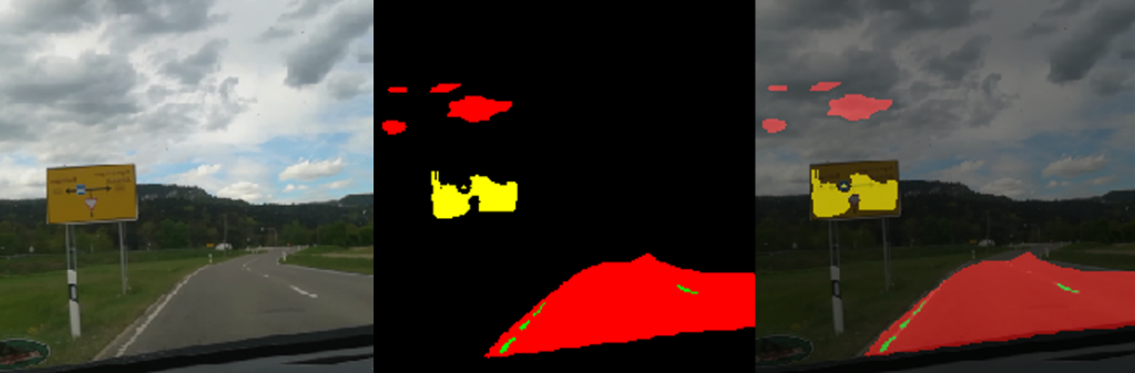
In Figure 4 you find one prediction from an original image. The original image is on the left side. The predicted mask in the middle, and the combined image on the right side.
Figure 4: Original image, predicted mask and overlaid image
You can see that the street was recognized pretty well, however parts of the sky was taken as a street as well. The traffic sign was labeled too, but not completely. As mentioned before we assume that we should have much more training data, to get better results.
Creating an augmented video
The code below creates an augmented video from an original video the students made in the beginning of the project. The name of the original video is video3.mp4. The name of the augmented video is videounet-3-drop.mp4. The method read of VideoCapture reads in each single images from video3.mp4 and stores them into the local variable frame. The image in frame is normalized and the mask image is predicted. The function predictedmask converts the mask into a 256×256 representation, and the function makemask creates a color image from it. Finally frame and the color mask are overlaid and saved to the new augmented video videounet-3-drop.mp4.
cap = cv2.VideoCapture(os.path.join(path,"videos",'video3.mp4'))
if (cap.isOpened() == True):

    print("Opening video stream or file")
    out = cv2.VideoWriter(os.path.join(path,"videos",'videounet-3-drop.mp4'),cv2.VideoWriter_fourcc(*'MP4V'), 25, (256,256))
    while(cap.isOpened()):
        ret, frame = cap.read()

        if ret == False:
            break

        test_data = []
        test_data.append(frame)
        test_data = np.array(test_data, dtype=np.float32)
        test_data /= 255.0

        predicted = model.predict(test_data, batch_size=1, verbose=0)
        assert(len(predicted) == 1)
        pmask = predictedmask(predicted)

        if ret == True:

            mask = makemask(pmask[0])

            weighted = np.zeros((dim[0], dim[1], 3), 'uint8')
            cv2.addWeighted(frame, 0.6, mask, 0.4, 0, weighted)


            out.write(weighted)
            cv2.imshow('Frame',weighted)
            if cv2.waitKey(25) & 0xFF == ord('q'):
                break

    out.release()

cap.release()
cv2.destroyAllWindows()
Conclusion
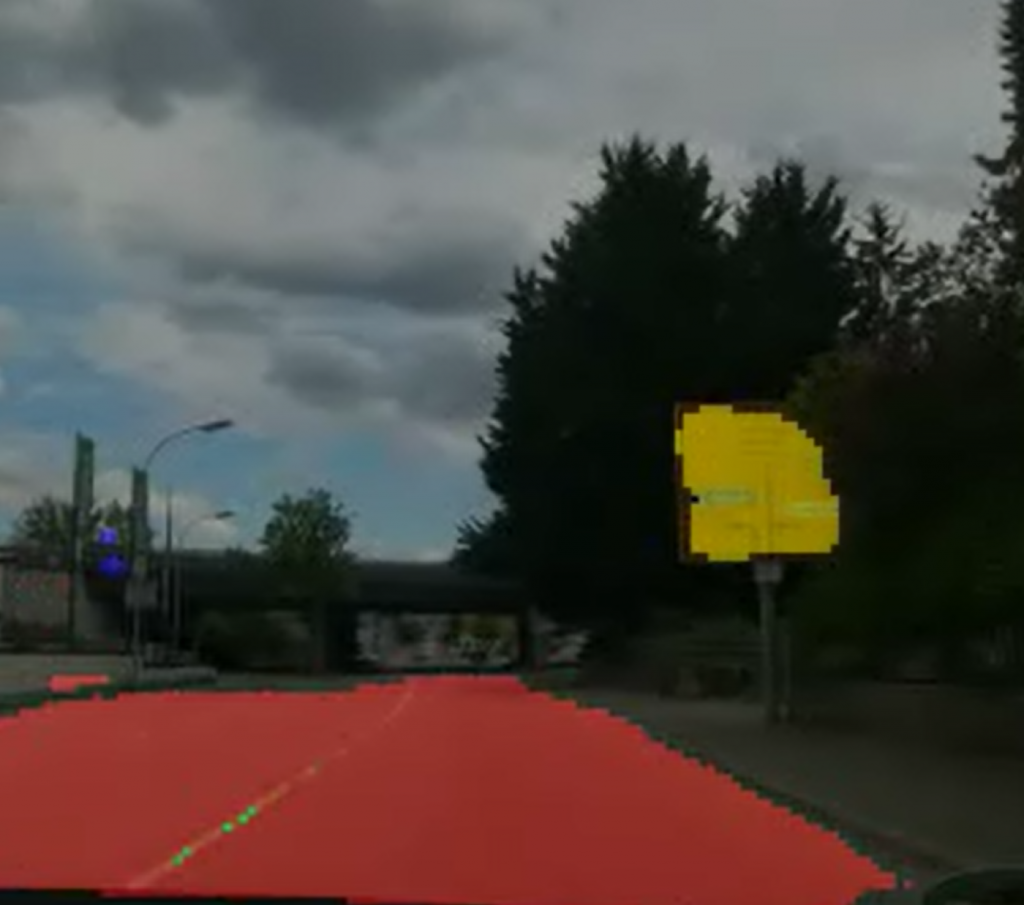
In Figure 5 you see a snapshot of the augmented video. The street is marked pretty well. You can even see how the sidewalk is not marked as a street. On the right side you find a traffic sign in yellow. The prediction works here good too. On the left side you find blue marking. The color blue categorizes cars. However there are no cars on the original image and therefore this is a misinterpretation. The street markings in green are not shown very well. In some parts of the augmented video they appear very strong, and in some parts you see only fragments, just like in Figure 5.
Figure 5: Snapshot of the augmented video
Overall we are very happy with the result of this project, considering that we have only labeled 250 images. We are convinced that we get better results as soon as we have more images for training. To overcome the problem we tried with data augmentation. So from the 250 images we created around 3000 images. We also randomly flipped the images horizontally in a code version, which was not discussed here.
We think that we have too much overfitting, which can only be solved with more training data. Due to the time limit, we had to restrict ourselves with fewer training data.
Acknowledgement
Special thanks to the class of Summer Semester 2020 Design Cyber Physical Systems providing the videos while driving and labeling the images for the training data used for the neural network. We appreciate this very much since this is a lot of effort.
Also special thanks to the University of Applied Science Albstadt-Sigmaringen for providing the infrastructure and the appliances to enable this class and this research.
As a instructor I offer a class, in which I let master students choose a topic for practical work during a semester. I usually give them a rough description, which included last time a raspberry pi, a camera, and a neural network.
Some students have chosen to work on fruit recognition with a camera. So the scenario is the following: The camera is connected to a raspberry pi. The camera observes a clean table. As soon as a user puts a fruit onto the table, the user can hit a button on a shield attached on the raspberry pi. The button triggers the camera to take an image. Then, the image is fed into a trained neural network for image categorization. The category was then fed into a speech synthesizer to speak out the category.
The type of neural network my students and I used is a multi-categorical neuronal network. So the goal was to feed the neuronal network with image and a category will come out as an output.
Preparing the Data
In the beginning we chose fruit images from a database which is available on github. You find it here. It had about 120 different categories of fruits and vegetables available. The problem we find with these images are, that the fruits and vegetables seemed to be perfect looking which is in reality not the case. The variation of fruit images within one category also seemed to be very limited. On the one hand, they do have many images within each category, on the other hand it looks like each image from one category only comes from a perfect fruit photographed in different positions.
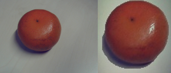
The fruits fill out the complete image, as well. When you photograph a fruit from a table, this is in general not the case. The left part of Figure 1 shows an orange which fills in only part of the image.
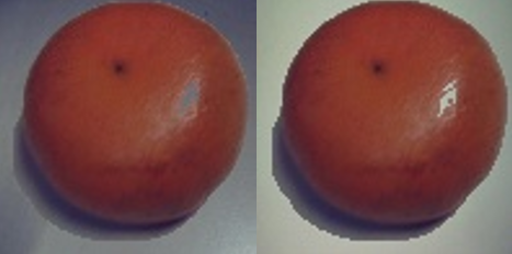
What is more, the background of the images from the database is extremely bright. This is not quite a real life background, which we find is much darker when you take pictures from inside a building. In Figure 2 you can see two different backgrounds which are surfaces from two different tables. The backgrounds do have relatively low brightness.
Cropping the images
The first task was to prepare the data for training the neural network. We decided to crop the images to the size of the fruits, so we receive some kind of standardization of the images. Below you find the code which crops the images to the size of the fruit. In this case we have the fruit images inside the addfolder. Inside the addfolder we first have two more directories, Testing and Training. Below these directories you find the directories for each fruit. We limit the number of fruits to six. The fruits we use are listed in dirlist, which are also the directory names.
The code is iterating through the Testing and Training directories and the fruit directories in dirlist and loads in every image with the opencv function imread. It converts the loaded image to a grayscale image and filters it with the opencv threshold function. After this we apply the findContours function which returns a list of contours of the image. The second largest contour (the largest contour has the size of the image itself) is taken and the width and height information of the contour is retrieved. The second largest contour is the fruit portion on the image. The application copies a square at the position of the second largest contour from the original image, resizes it to 100×100 pixels and saves it into a new directory destfolder.
srcfolder = '/home/inf/Bilder/Scale/orig/'
destfolder = '/home/inf/Bilder/Scale/cropped/'
addfolder = '/home/inf/Bilder/Scale/added/'
processedfolder = '/home/inf/Bilder/Scale/processed/'

dirtraintest = ['Testing', 'Training']
dirlist = ['Apfel','Gurke','Kartoffel','Orange','Tomate','Zwiebel']

count = 0
pattern = "*.jpg"
img_size = (100,100)

for traintest in dirtraintest:
    for fruit in dirlist:
        count = 0
        for file in glob.glob(os.path.join(addfolder, traintest, fruit, pattern)):
            im = cv2.imread(file)
            imgray = cv2.cvtColor(im, cv2.COLOR_BGR2GRAY)
            ret, thresh = cv2.threshold(imgray, 127, 200, 0)
            contours, hierarchy = cv2.findContours(thresh, cv2.RETR_TREE, cv2.CHAIN_APPROX_SIMPLE)
            if len(contours) > 1:
                cnt = sorted(contours, key=cv2.contourArea)
                x, y, w, h = cv2.boundingRect(cnt[-2])
                w = max((h, w))
                h = w
                crop_img = im[y:y+h, x:x+w]
            im = cv2.resize(crop_img, img_size)
            cv2.imwrite(os.path.join(destfolder, traintest, fruit, str("cropped_img_"+str(count)+".jpg")), im)
            count += 1
Figure 1 shows how the application crops an image of an orange. On the left side, the orange fills out only part of the image. On the right side, the orange fills out the complete image.
Figure 1: Original Image and Cropped Image
Changing the backgrounds
Due to the extreme bright background of the images from the database we came to the decision to fill in new backgrounds on top of the bright ones. In Figure 2, you can see two different table surfaces, taken by the camera we used.
Figure 2: Backgrounds
The code below shows how each image from the directory structure (which I explained above) is loaded into the variable pixels with the opencv imread function. Each pixel on each layer (RGB) of the image is checked, if a threshold of brightness has been reached. We assume that a pixel exceeding a certain brightness threshold is a background pixel (which is not always the case). The application then replaces the pixel with a pixel from a background image shown in Figure 2. It saves the new image to the directory processedfolder.
background = cv2.imread("background.jpg")

bg = np.zeros((img_size[0], img_size[1],3), np.uint8)
bgData = np.zeros((img_size[0], img_size[1],3), np.uint8)

bg = cv2.resize(background, img_size)
bgData = bg.copy()

threshold = (100, 100, 100)

for traintest in dirtraintest:
    for fruit in dirlist:
        count = 0
        for name in glob.glob(os.path.join(destfolder, traintest, fruit, pattern)):
            pixels = cv2.imread(os.path.join(destfolder, traintest, fruit, name))
            pixelsData = pixels.copy()

            for i in range(pixels.shape[0]): # for every pixel:
                for j in range(pixels.shape[1]):
                    if pixelsData[i, j][0] >= threshold[0] and pixelsData[i, j][1] >= threshold[1] and pixelsData[i, j][2] >= threshold[2]:
                        pixelsData[i, j] = bgData[i, j]
            cv2.imwrite(os.path.join(processedfolder, traintest, fruit, str("processed_img_"+str(count)+".jpg")), pixelsData)
            count += 1
Figure 3 shows the output of two images from the code above. It shows the same orange with two different backgrounds.
Figure 3: Orange with two different Backgrounds
Training the Model
Below the code of a neural network model. It consists of four convolutional layers. The number of filters is increased with each layer. After each convolutional layer there is a max pooling layer to reduce the image size for the input of the following layer. A flatten layer follows and is fed into a dense layer. Finally there is another dense layer with six neurons. This is the number of categories we have. Each layer uses the relu activation function. In the last layer however we use the softmax activation function. The reason for softmax, and not sigmoid, is, that we expect only one category from the six categories to be true for a given input image. This can be represented by the highest number calculated from the six output neurons. For optimization, we use stochastic gradient descent method.
We load in all training and validation images from the directory train_path and valid_path with the Keras ImageDataGenerator. By doing this the ImageDataGenerator rescales the images and augment the images by shifting and flipping. The training and validation images from the directories train_path and valid_path are moved into the lists train_it and valid_it. The method flow_from_directory makes this task easy since it considers the directory structure below the directories train_path and valid_path, as well. In our case, we have the directories Apfel, Gurke, Kartoffel, Orange, Tomate, Zwiebel below of train_path and valid_path. In each of these directories you find the corresponding images (such all apple images in directory Apfel, all cucumber images in directory Gurke etc.).
The training is started with the Keras fit_generator command. It uses the lists train_it and valid_it as inputs. We defined a callback function to produce checkpoints from the neural network weights, each time the training shows some improvement concerning validation loss.
Finally the structure of the trained model is saved to a json file.
The training time with this model is about three minutes on a NVIDIA graphics card. We use about 6000 images for training and 2000 images for validation, altogether. The validation accuracy was 96% which was above the accuracy, which shows a little underfitting.
Testing the Model
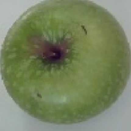
We tested the model with the code below. First, we loaded the image in the variable img with the opencv function imread read. Right after this, we have to take care of the image layers. The way opencv handles the image layers is different from the way Keras with its predict method does. They have the Red and the Blue layers switched. For this reason, we have to apply the cvtColor method, which switches the Red and Blue layers. The image is then normalized by dividing its pixels values with 255. Finally the prediction method is used to predict the image. Figure 4 shows an example of an image for input, which is printed out by the matplotlib function imshow. The method predict returns a probability vector predictions. The index with the highest value of the vector corresponds to the category. The category can be retrieved from the class_indices list.
We tested a few times with different image and saw that the prediction delivered pretty good results.
Figure 4: Prediction Image
The Raspberry Pi application
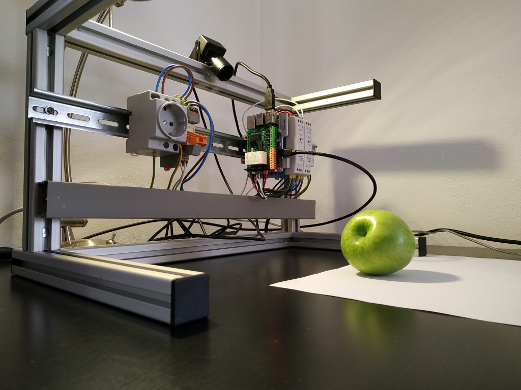
The setup of the experiment is shown in Figure 5. The raspberry pi 4, power supply and a socket are mounted on a top-hat rail. On the raspberry pi you see a piface shield attached. The shield had to be mechanically prepared to fit on a raspberry pi 4. The shield provides buttons in case it is needed. Additionally we have a relay and a power socket. The relay can be triggered by the piface, so the relay applies 230V to the socket. On top of the construction you find an usb camera.
Figure 5: Experiment Setup
We defined a function getCrop, see code below, which crops the image to the size of the portion of the fruit. This procedure was already explained above. Here we introduced the variable threshset, where the user can modify the threshold value of the opencv threshold method using keys. This is explained later.
threshset = 100

def getCrop(im):
    global threshset
    imgray = cv2.cvtColor(im, cv2.COLOR_BGR2GRAY)
    ret, thresh = cv2.threshold(imgray, threshset, 255, 0)
    contours, hierarchy = cv2.findContours(thresh, cv2.RETR_TREE, cv2.CHAIN_APPROX_SIMPLE)
    if len(contours) >= 1:
        cnts = sorted(contours, key=cv2.contourArea, reverse=True)
        for cnt in cnts:
            x, y, w, h = cv2.boundingRect(cnt)
            if w > im.shape[0]*20//100 and w < im.shape[0]*95//100:
                if h > im.shape[1]*20//100 and h < im.shape[1]*95//100:
                    w = max((h, w))
                    h = w
                    return x,y,w
    return 0,0,0
In the beginning we faced the problem that the neural network did not predict very well due to too few training images. Therefore we introduced a function to save easily badly predicted images. The name of the function is saveimg. It simply saves an image img to a directory with a name containing the parameters dircat and fruit. The image name also contains the date and the time.
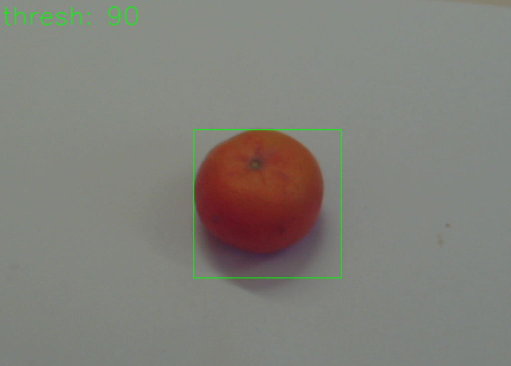
Below you find the raspberry pi application code. In the beginning it sets up the opencv video feature. Inside the while loop, an image frame from the usb camera is taken, which is then copied into the image objectfr. The function getCrop is used to get the fruit portion of the image and a rectangle is drawn around the fruit portion. The function putText writes the current value of threshset into the image objectfr as well. The application then shows the modified image on a display, see Figure 6. The opencv method waitkey checks for a pressed key. In case a key was pressed, code depending on the key will be executed.
If the key ‘q’ is pressed, than the application stops. If the key ‘n’ is pressed, the image inside the rectangle is taken and the category is predicted with the Keras predict method. The string is handed over to the espeak application which speaks out the category on the speaker attached on the raspberry pi. The keys ‘a’, ‘z’, ‘o’, ‘k’ execute the saveimg function with different parameters. The purpose of these keys is, that the user can save an image, in case there is a bad prediction. Next time, the model is trained, the saved image will be included in the training data. At last we have the ‘+’ and ‘-‘ keys, which modify the threshset value. The effect will be, that the rectangle (Figure 6, green rectangle) is enlarged or downsized due to the shadow on the background.
Figure 6: Displayed Image
Conclusion
The application works amazingly well with few fruits to predict considering the relative low number of training data. In the beginning we had to retrain the model a couple of times with newly generated images using the application keys described above.
As soon as we take e.g. an apple with different colors, there is a high chance that the prediction fails. In such cases we have take more images and retrain again.
Acknowledgement
Thanks to Carmen Furch and Armin Weisser providing the data preparation code and the raspberry pi application.
Also special thanks to the University of Applied Science Albstadt-Sigmaringen offering a classroom and appliances to enable this research.