Street Scene Segmentation with a UNET-Model

For the summer semester 2020 we offered an elective class called Design Cyber Physical Systems. This time only few students enrolled into the class. The advantage of having small classes is that we can focus on a certain topic without loosing the overview during project execution. The class starts with a brain storming session to choose a topic to be worked on during the semester. There are only a few constraints which we ask to apply. The topic must have something to do with image processing, neural networks and deep learning. The students came up with five ideas and presented them to the instructor. The instructor commented on the ideas and evaluated them. Finally the students chose one of the idea to work on until the end of the semester.

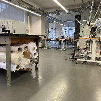
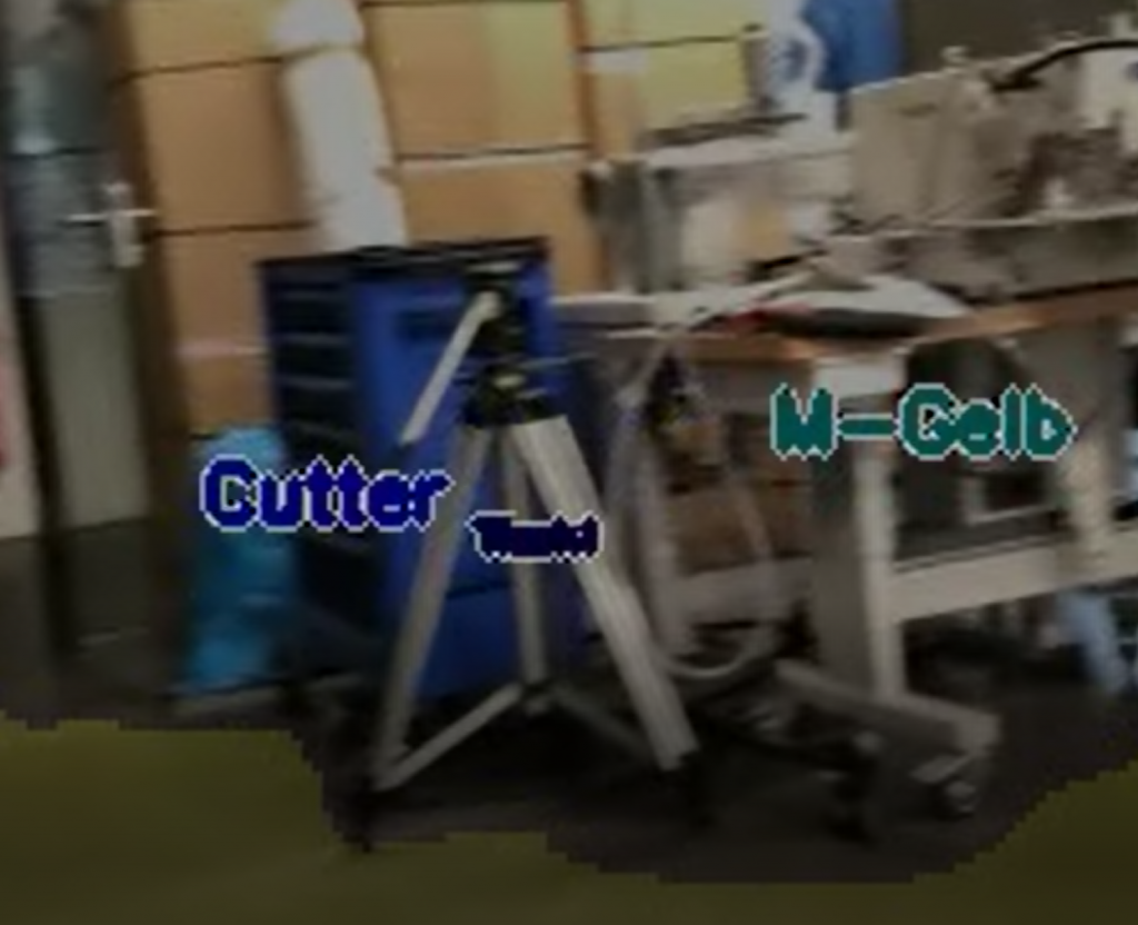
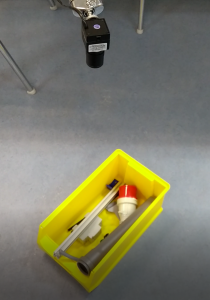
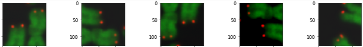
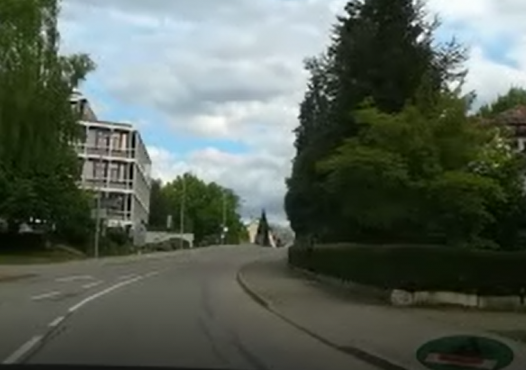
This time the students chose to process street scenes taken from videos while driving a car. A street scene can be seen in Figure 1. The videos were taken in driving direction through the front window of a car. The assignment the students have given to themselves is to extract street, street marking, traffic signs, and cars on the video images. This kind of problem is called semantic segmentation, which has been solved in a similar fashion as in the previous post. Therefore many functions in this post and in the last post are pretty similar.

Figure 1: Street scene

Creating Training Data

The students took about ten videos while driving a car to create the training data. Since videos are just a sequence of images, they selected randomly around 250 images from the videos. Above we mentioned that we wanted to extract street, street marking, traffic signs and cars. These are four categories. There is another one, which is neither of those (or the background category). This makes it five categories. Below you find code of python dictionaries. The first is the dictionary classes which assigns text to the category numbers (such as the number 1 is assigned to Strasse (Street in English). The dictionary categories assigns it the way around. Finally the dictionary colors assigns a color to each category number.

classes = {"Strasse" : 1, 
           "strasse" : 1,
          "Streifen" : 2,
           "streifen" : 2,
          "Auto" : 3, 
          "auto" : 3,
          "Schild" : 4,
           "schild" : 4,
         }

categories = {1: "Strasse", 
              2: "Streifen",
              3: "Auto", 
              4: "Schild",           
         }

colors = {0 : (0,0,0), 
          1 : (0,0,255), 
          2 : (0,255,0),
          3 : (255,0,0), 
          4 : (0,255,255),         
         }

dim = (256, 256) 

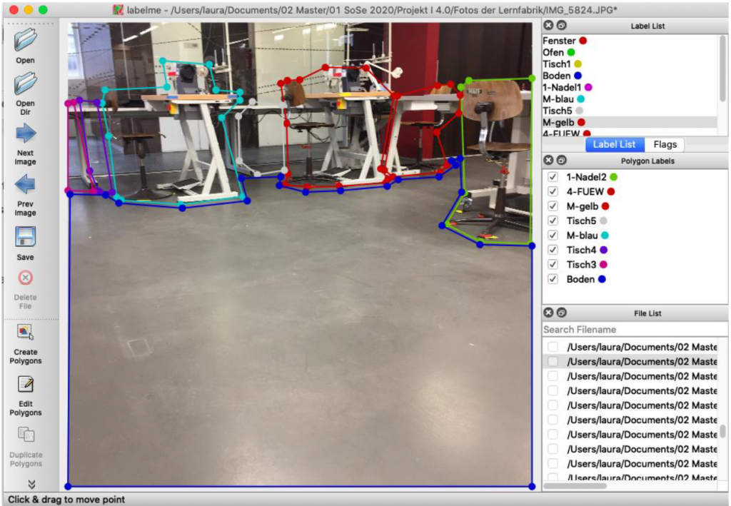
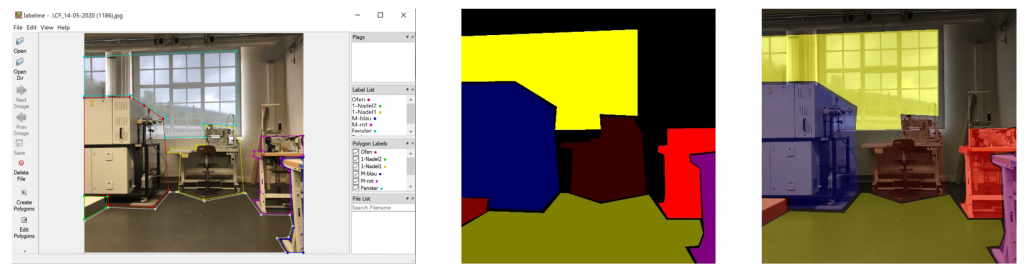
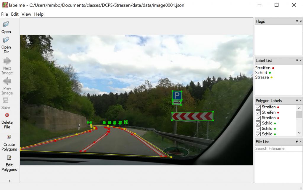
To create training data we decided to use the tool labelme, which is described here. You can load images into the tool, and mark regions by drawing polygons around them, see Figure 2. The regions can be categorized with a names which are the same as from the python dictionary categories, see code above. You can save the polygons, its categories and the image itself to a json file. Now it is very easy to parse the json file with a python parser.

Figure 2: Tool labelme

The image itself is stored in the json file in a base-64 representation. Here python has tools as well, to parse out the image. Videos generally do not store square images, so we need to convert them into a square image, which is better for training the neural network. We have written the following two functions to fulfill this task: makesquare2 and makesquare3. The difference of these functions is, that the first handles grayscale images and the second RGB images. Both functions just omits evenly the left and the right portion of the original video image to create a square image.

def makesquare2(img):
    
    assert(img.ndim == 2) 
    
    edge = min(img.shape[0],img.shape[1])
        
    img_sq = np.zeros((edge, edge), 'uint8')
    
    if(edge == img.shape[0]):
        img_sq[:,:] = img[:,int((img.shape[1] - edge)/2):int((img.shape[1] - edge)/2)+edge]
    else:
        img_sq[:,:,:] = img[int((img.shape[0] - edge)/2):int((img.shape[0] - edge)/2)+edge,:]

    assert(img_sq.shape[0] == edge and img_sq.shape[1] == edge)
    
    return img_sq
def makesquare3(img):
    
    assert(img.ndim == 3)
    
    edge = min(img.shape[0],img.shape[1])
        
    img_sq = np.zeros((edge, edge, 3), 'uint8')
    
    if(edge == img.shape[0]):
        img_sq[:,:,:] = img[:,int((img.shape[1] - edge)/2):int((img.shape[1] - edge)/2)+edge,:]
    else:
        img_sq[:,:,:] = img[int((img.shape[0] - edge)/2):int((img.shape[0] - edge)/2)+edge,:,:]

    assert(img_sq.shape[0] == edge and img_sq.shape[1] == edge)
    
    return img_sq

Below you see two functions createMasks and createMasksAugmented. We need the functions to create training data from the json files, such as original images and mask images. Both functions have been described in the post before. Therefore we dig only into the differences.

In both functions you find a special handling for the category Strasse (Street in English). You can find it below the code snippet:

classes[shape[‘label’]] != classes[‘Strasse’]

Regions in the images, which are marked as Strasse (Street in English) can share the same region as Streifen (Street Marking in English) or Auto (Car in English). We do not want that street regions overrule the street marking or car regions, otherwise the street marking or the cars will disappear. For this we create first a separate mask mask_strasse. All other category masks are substracted from mask_strasse, and then mask_strasse is added to the finalmask. Again, we just want to make sure that the street marking mask and the other masks are not overwritten by the street mask.

def createMasks(sourcejsonsdir, destimagesdir, destmasksdir):

    assocf = open(os.path.join(path,"assoc_orig.txt"), "w")
    count = 0
    directory = sourcejsonsdir
    for filename in os.listdir(directory):
        if filename.endswith(".json"):
            print("{}:{}".format(count,os.path.join(directory, filename)))
            
            f = open(os.path.join(directory, filename))
            data = json.load(f)
            img_arr = data['imageData']  
            imgdata = base64.b64decode(img_arr)

            img = cv2.imdecode(np.frombuffer(imgdata, dtype=np.uint8), flags=cv2.IMREAD_COLOR)
            
            assert (img.shape[0] > dim[0])
            assert (img.shape[1] > dim[1])
           
            finalmask = np.zeros((img.shape[0], img.shape[1]), 'uint8')
        
            masks=[]
            masks_strassen=[]
            mask_strasse = np.zeros((img.shape[0], img.shape[1]), 'uint8')
            
            for shape in data['shapes']:
                assert(shape['label'] in classes)

                vertices = np.array([[point[1],point[0]] for point in shape['points']])
                vertices = vertices.astype(int)

                rr, cc = polygon(vertices[:,0], vertices[:,1], img.shape)
                mask_orig = np.zeros((img.shape[0], img.shape[1]), 'uint8')

                mask_orig[rr,cc] = classes[shape['label']]
                if classes[shape['label']] != classes['Strasse']:
                    masks.append(mask_orig)
                else:
                    masks_strassen.append(mask_orig)
                    
            for m in masks_strassen:
                mask_strasse += m
                    
            for m in masks:
                _,mthresh = cv2.threshold(m,0,255,cv2.THRESH_BINARY_INV)
                finalmask = cv2.bitwise_and(finalmask,finalmask,mask = mthresh)
                finalmask += m

            _,mthresh = cv2.threshold(finalmask,0,255,cv2.THRESH_BINARY_INV)
            mask_strasse = cv2.bitwise_and(mask_strasse,mask_strasse, mask = mthresh)
            finalmask += mask_strasse  
                
            img = makesquare3(img)
            finalmask = makesquare2(finalmask)

            img_resized = cv2.resize(img, dim, interpolation = cv2.INTER_NEAREST)
            finalmask_resized = cv2.resize(finalmask, dim, interpolation = cv2.INTER_NEAREST)
            
            filepure,extension = splitext(filename)
            
            cv2.imwrite(os.path.join(destimagesdir, "{}o.png".format(filepure)), img_resized)
            cv2.imwrite(os.path.join(destmasksdir, "{}o.png".format(filepure)), finalmask_resized)

            assocf.write("{:05d}o:{}\n".format(count,filename))
            assocf.flush()
            count += 1

        else:
            continue
    f.close()

In createMask you find the usage of makesquare3 and makesquare2, since the video images are not square. However we prefer to use square image for neural network training.

def createMasksAugmented(ident, sourcejsonsdir, destimagesdir, destmasksdir):

    assocf = open(os.path.join(path,"assoc_{}_augmented.txt".format(ident)), "w")

    count = 0
    directory = sourcejsonsdir
    for filename in os.listdir(directory):
        if filename.endswith(".json"):
            print("{}:{}".format(count,os.path.join(directory, filename)))

            f = open(os.path.join(directory, filename))
            data = json.load(f)

            img_arr = data['imageData']  
            imgdata = base64.b64decode(img_arr)

            img = cv2.imdecode(np.frombuffer(imgdata, dtype=np.uint8), flags=cv2.IMREAD_COLOR)
            
            assert (img.shape[0] > dim[0])
            assert (img.shape[1] > dim[1])
            
            zoom = randint(75,90)/100.0
            angle = (2*random()-1)*3.0
            img_rotated = imutils.rotate_bound(img, angle)
            
            xf = int(img_rotated.shape[0]*zoom)
            yf = int(img_rotated.shape[1]*zoom)            
            
            img_zoomed = np.zeros((xf, yf, img_rotated.shape[2]), 'uint8')
            img_zoomed[:,:,:] = img_rotated[int((img_rotated.shape[0]-xf)/2):int((img_rotated.shape[0]-xf)/2)+xf,int((img_rotated.shape[1]-yf)/2):int((img_rotated.shape[1]-yf)/2)+yf,:] 
        

            finalmask = np.zeros((img_zoomed.shape[0], img_zoomed.shape[1]), 'uint8')
            mthresh = np.zeros((img_zoomed.shape[0], img_zoomed.shape[1]), 'uint8')
            masks=[]
            masks_strassen=[]
            mask_strasse = np.zeros((img_zoomed.shape[0], img_zoomed.shape[1]), 'uint8')

            for shape in data['shapes']:
                assert(shape['label'] in classes)

                vertices = np.array([[point[1],point[0]] for point in shape['points']])
                vertices = vertices.astype(int)

                rr, cc = polygon(vertices[:,0], vertices[:,1], img.shape)
                mask_orig = np.zeros((img.shape[0], img.shape[1]), 'uint8')
                mask_orig[rr,cc] = classes[shape['label']]
                
                mask_rotated = imutils.rotate_bound(mask_orig, angle)
                
                mask_zoomed = np.zeros((xf, yf), 'uint8')
                mask_zoomed[:,:] = mask_rotated[int((img_rotated.shape[0]-xf)/2):int((img_rotated.shape[0]-xf)/2)+xf,int((img_rotated.shape[1]-yf)/2):int((img_rotated.shape[1]-yf)/2)+yf] 
                
                if classes[shape['label']] != classes['Strasse']:
                    masks.append(mask_zoomed)
                else:
                    masks_strassen.append(mask_zoomed)

            for m in masks_strassen:
                mask_strasse += m
                    
            for m in masks:
                _,mthresh = cv2.threshold(m,0,255,cv2.THRESH_BINARY_INV)
                finalmask = cv2.bitwise_and(finalmask,finalmask,mask = mthresh)
                finalmask += m

            _,mthresh = cv2.threshold(finalmask,0,255,cv2.THRESH_BINARY_INV)
            mask_strasse = cv2.bitwise_and(mask_strasse,mask_strasse, mask = mthresh)
            finalmask += mask_strasse    
    
            # contrast-> alpha: 1.0 - 3.0; brightness -> beta: 0 - 100
            alpha = 0.8 + 0.4*random();
            beta = int(random()*15)
    
            img_adjusted = cv2.convertScaleAbs(img_zoomed, alpha=alpha, beta=beta)
        
        
            img_adjusted = makesquare3(img_adjusted)
            finalmask = makesquare2(finalmask)

            img_resized = cv2.resize(img_adjusted, dim, interpolation = cv2.INTER_NEAREST)
            finalmask_resized = cv2.resize(finalmask, dim, interpolation = cv2.INTER_NEAREST)
            
            filepure,extension = splitext(filename)
            
            if randint(0,1) == 0:
                cv2.imwrite(os.path.join(destimagesdir, "{}{}.png".format(filepure, ident)), img_resized)
                cv2.imwrite(os.path.join(destmasksdir, "{}{}.png".format(filepure, ident)), finalmask_resized) 
            else:
                cv2.imwrite(os.path.join(destimagesdir, "{}{}.png".format(filepure, ident)), cv2.flip(img_resized,1))
                cv2.imwrite(os.path.join(destmasksdir, "{}{}.png".format(filepure, ident)), cv2.flip(finalmask_resized,1))    
                
            assocf.write("{:05d}:{}\n".format(count, filename))
            assocf.flush()
            count += 1

        else:
            continue
    f.close()

The function createMasksAugmented above does basically the same thing as createMasks, but the image is randomly zoomed and rotated. Also the brightness and contrast is randomly adjusted. The purpose is to create more varieties of images from the original image for regularization.

The original images and mask images for neural network training can be generated by calling the functions below. In the directory fullpathjson you find the source json files. The parameters fullpathimages and fullpathmasks are the directory names for the destination.

Since we labeled 250 video images and stored them to json files, the functions below create altogether 1000 original and mask images. The function createMasksAugmented can be called even more often for more data.

createMasks(fullpathjson, fullpathimages, fullpathmasks)
createMasksAugmented("a4",fullpathjson, fullpathimages, fullpathmasks)
createMasksAugmented("a5",fullpathjson, fullpathimages, fullpathmasks)
createMasksAugmented("a6",fullpathjson, fullpathimages, fullpathmasks)

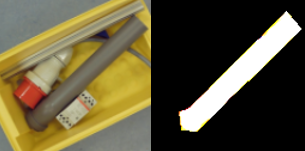
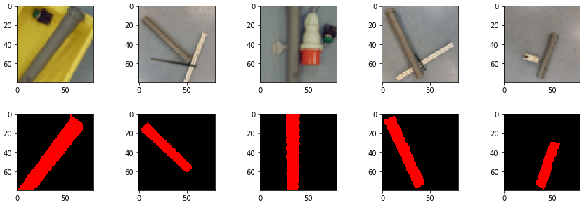
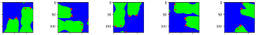
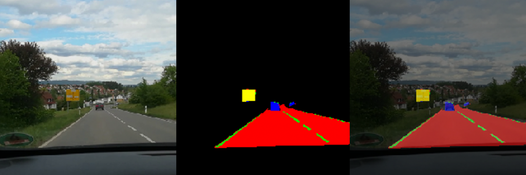
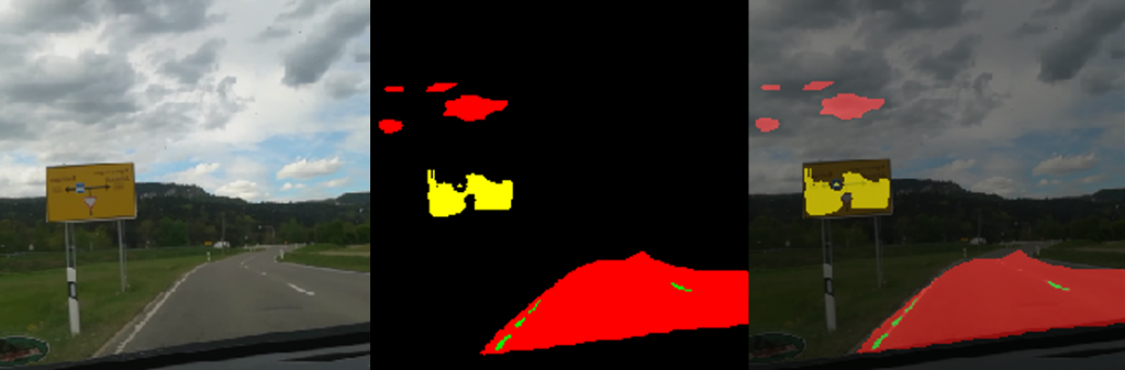
In Figure 3 below you find one result of the applied createMasks function. Left, there is an original image. In the middle there is the corresponding mask image. On the right there is the overlaid image. The region of the traffic sign is marked yellow, the street has color red, the street marking is in green and finally the car has a blue color.

Figure 3: Original Image, mask image and overlaid image

Training the model

We used different kinds of UNET models and compared the results from them. The UNET model from the previous post had mediocre results. For this reason we switched to an UNET model from a different author. It can be found here. The library keras_segmentation gave us much better predictions. However we do not have so much control over the model itself, for this was the reason we created our own UNET model, but we were inspired by keras_segmentation.

Above we already stated that we have five categories. Each category gets a number and a color assigned. The assignment can be seen in the python dictionary below.

colors = {0 : (0,0,0), 
          1 : (0,0,255), 
          2 : (0,255,0),
          3 : (255,0,0), 
          4 : (0,255,255),         
         }


dim = (256, 256) 

The UNET model we created is shown in the code below. It consists of a contracting and an expanding path. In the expanding path we have five convolution operations, followed by batch normalizations, relu-activations and maxpoolings. In between we also use dropouts for regularization. The results of these operations are saved into variables (c0, c1, c2, c3, c4). In the expanding path we implemented the upsampling operations and concatenate their outputs with the variables (c0, c1, c2, c3, c4) from the contracting path. Finally the code performs a softmax operation.

In general the concatenation of the outputs with the variables show benefits during training. Gradients of upper layers often vanish during the backpropagation operation. Concatenation is the method to prevent this behavior. However if this is really the case here has not been proofed.

def my_unet(classes):
    
    dropout = 0.4
    input_img = Input(shape=(dim[0], dim[1], 3))
    
    #contracting path
    x = (ZeroPadding2D((1, 1)))(input_img)
    x = (Conv2D(64, (3, 3), padding='valid'))(x)
    x = (BatchNormalization())(x)
    x = (Activation('relu'))(x)
    x = (MaxPooling2D((2, 2)))(x)
    c0 = Dropout(dropout)(x)
    
    x = (ZeroPadding2D((1, 1)))(c0)
    x = (Conv2D(128, (3, 3),padding='valid'))(x)
    x = (BatchNormalization())(x)
    x = (Activation('relu'))(x)
    x = (MaxPooling2D((2, 2)))(x)
    c1 = Dropout(dropout)(x)

    x = (ZeroPadding2D((1, 1)))(c1)
    x = (Conv2D(256, (3, 3), padding='valid'))(x)
    x = (BatchNormalization())(x)
    x = (Activation('relu'))(x)
    x = (MaxPooling2D((2, 2)))(x)
    c2 = Dropout(dropout)(x)
    
    x = (ZeroPadding2D((1, 1)))(c2)
    x = (Conv2D(256, (3, 3), padding='valid'))(x)
    x = (BatchNormalization())(x)
    x = (Activation('relu'))(x)
    x = (MaxPooling2D((2, 2)))(x)
    c3 = Dropout(dropout)(x)
    
    x = (ZeroPadding2D((1, 1)))(c3)
    x = (Conv2D(512, (3, 3), padding='valid'))(x)
    c4 = (BatchNormalization())(x)

    #expanding path
    x = (UpSampling2D((2, 2)))(c4)
    x = (concatenate([x, c2], axis=-1))
    x = Dropout(dropout)(x)
    x = (ZeroPadding2D((1, 1)))(x)
    x = (Conv2D(256, (3, 3), padding='valid', activation='relu'))(x)
    e4 = (BatchNormalization())(x)
    
    x = (UpSampling2D((2, 2)))(e4)
    x = (concatenate([x, c1], axis=-1))
    x = Dropout(dropout)(x)
    x = (ZeroPadding2D((1, 1)))(x)
    x = (Conv2D(256, (3, 3), padding='valid', activation='relu'))(x)
    e3 = (BatchNormalization())(x)
    
    x = (UpSampling2D((2, 2)))(e3)
    x = (concatenate([x, c0], axis=-1))
    x = Dropout(dropout)(x)
    x = (ZeroPadding2D((1, 1)))(x)
    x = (Conv2D(64, (3, 3), padding='valid', activation='relu'))(x)
    x = (BatchNormalization())(x)

    x = (UpSampling2D((2, 2)))(x)
    x = Conv2D(classes, (3, 3), padding='same')(x)
    
    x = (Activation('softmax'))(x)
    
    model = Model(input_img, x)
        
    return model

As described in the last post, we use for training a different kind of mask representation than the masks created by createMasks. In our case, the UNET model needs masks in the shape 256x256x5. The function createMasks creates masks in shape 256×256 though. For training it is preferable to have one layer for each category. This is why we implemented the function makecolormask. It is the same function as described in the last post, but it is optimized and performs better. See code below.

def makecolormask(mask):
    ret_mask = np.zeros((mask.shape[0], mask.shape[1], len(colors)), 'uint8')
    
    for col in range(len(colors)):
        ret_mask[:, :, col] = (mask == col).astype(int)
                       
    return ret_mask

Below we define callback functions for the training period. The callback function EarlyStopping stops the training after ten epoch if there is no improvement concerning validation loss. The callback function ReduceLROnPlateau reduces the learning rate if there is no improvement concerning validation loss after three epochs. And finally the callback function ModelCheckpoint creates a checkpoint from the UNET model’s weights, as soon as an improvement of the validation loss has been calculated.

modeljsonname="model-chkpt.json"
modelweightname="model-chkpt.h5"

callbacks = [
    EarlyStopping(patience=10, verbose=1),
    ReduceLROnPlateau(factor=0.1, patience=3, min_lr=0.00001, verbose=1),
    ModelCheckpoint(os.path.join(path, dirmodels,modelweightname), verbose=1, save_best_only=True, save_weights_only=True)
]

The code below is used to load batches of original images and mask images into lists, which are fed into the training process. The function generatebatchdata has been described last post, so we omit the description since it is nearly identical.

def generatebatchdata(batchsize, fullpathimages, fullpathmasks):
  
    imagenames = os.listdir(fullpathimages)
    imagenames.sort()

    masknames = os.listdir(fullpathmasks)
    masknames.sort()

    assert(len(imagenames) == len(masknames))
    
    for i in range(len(imagenames)):
        assert(imagenames[i] == masknames[i])

    while True:
        batchstart = 0
        batchend = batchsize    
        
        while batchstart < len(imagenames):
            
            imagelist = []
            masklist = []
            
            limit = min(batchend, len(imagenames))

            for i in range(batchstart, limit):
                if imagenames[i].endswith(".png"):
                    imagelist.append(cv2.imread(os.path.join(fullpathimages,imagenames[i]),cv2.IMREAD_COLOR ))
                if masknames[i].endswith(".png"):
                    masklist.append(makecolormask(cv2.imread(os.path.join(fullpathmasks,masknames[i]),cv2.IMREAD_UNCHANGED )))


            train_data = np.array(imagelist, dtype=np.float32)
            train_mask= np.array(masklist, dtype=np.float32)

            train_data /= 255.0
    
            yield (train_data,train_mask)    

            batchstart += batchsize   
            batchend += batchsize

The variables generate_train and generate_valid are instantiated from generatebatchdata below. We use a batch size of two. We had trouble with a breaking the training process, as soon as the batch size was too large. We assume it is because of memory overflow in the graphic card. Setting it to a lower number worked fine. The method fit_generator starts the training process. The training took around ten minutes on a NVIDIA 2070 graphic card. The accuracy has reached 98% and the validation accuracy has reached 94%. This is pretty much overfitting, however we are aware, that we have very few images to train. Originally we created only 250 masks from the videos in the beginning. The rest of the training data resulted from data augmentation.

generator_train = generatebatchdata(2, fullpathimages, fullpathmasks)
generator_valid = generatebatchdata(2, fullpathimagesvalid, fullpathmasksvalid)
model.fit_generator(generator_train,steps_per_epoch=700, epochs=10, callbacks=callbacks, validation_data=generator_valid, validation_steps=100)

After training we saved the model. First the model structure is saved to a json file. Second the weights are saved by using the save_weights method.

model_json = model.to_json()
with open(os.path.join(path, dirmodels,modeljsonname), "w") as json_file:
    json_file.write(model_json)

model.save_weights(os.path.join(path, dirmodels,modelweightname))

The predict method of the model predicts masks from original images. It returns a list of masks, see code below. The parameter test_data is a list of original images.

predictions_test = model.predict(test_data, batch_size=1, verbose=1)

The masks in predictions_test from the model prediction have a 256x256x5 shape. Each layer represents a category. It is not convenient to display this mask, so predictedmask converts it back to a 256×256 representation. The code below shows predictedmask.

def predictedmask(masklist):
    y_list = []
    for mask in masklist:
        assert mask.shape == (dim[0], dim[1], len(colors))
        imgret = np.zeros((dim[0], dim[1]), np.uint8)
        
        imgret = mask.argmax(axis=2)
        
        y_list.append(imgret)
                    
    return y_list

Another utility function for display purpose is makemask, see code below. It converts 256×256 mask representation to a color mask representation by using the python dictionary colors. Again this is a function from last post, however optimized for performance.

def makemask(mask):
    ret_mask = np.zeros((mask.shape[0], mask.shape[1], 3), 'uint8')

    for col in range(len(colors)):
        layer = mask[:, :] == col
        ret_mask[:, :, 0] += ((layer)*(colors[col][0])).astype('uint8')
        ret_mask[:, :, 1] += ((layer)*(colors[col][1])).astype('uint8')
        ret_mask[:, :, 2] += ((layer)*(colors[col][2])).astype('uint8')
    
    return ret_mask

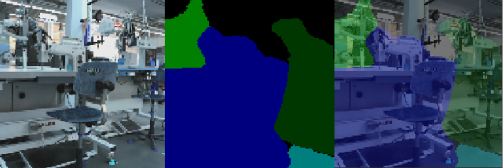
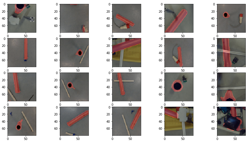
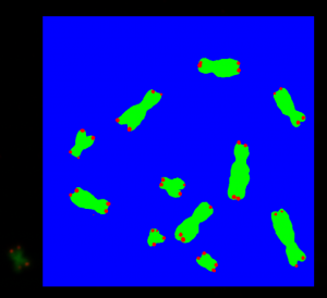
In Figure 4 you find one prediction from an original image. The original image is on the left side. The predicted mask in the middle, and the combined image on the right side.

Figure 4: Original image, predicted mask and overlaid image

You can see that the street was recognized pretty well, however parts of the sky was taken as a street as well. The traffic sign was labeled too, but not completely. As mentioned before we assume that we should have much more training data, to get better results.

Creating an augmented video

The code below creates an augmented video from an original video the students made in the beginning of the project. The name of the original video is video3.mp4. The name of the augmented video is videounet-3-drop.mp4. The method read of VideoCapture reads in each single images from video3.mp4 and stores them into the local variable frame. The image in frame is normalized and the mask image is predicted. The function predictedmask converts the mask into a 256×256 representation, and the function makemask creates a color image from it. Finally frame and the color mask are overlaid and saved to the new augmented video videounet-3-drop.mp4.

cap = cv2.VideoCapture(os.path.join(path,"videos",'video3.mp4'))
if (cap.isOpened() == True): 
    
    print("Opening video stream or file")
    out = cv2.VideoWriter(os.path.join(path,"videos",'videounet-3-drop.mp4'),cv2.VideoWriter_fourcc(*'MP4V'), 25, (256,256))
    while(cap.isOpened()):
        ret, frame = cap.read()
        
        if ret == False:
            break

        test_data = []
        test_data.append(frame)
        test_data = np.array(test_data, dtype=np.float32)
        test_data /= 255.0
        
        predicted = model.predict(test_data, batch_size=1, verbose=0)
        assert(len(predicted) == 1)
        pmask = predictedmask(predicted)
        
        if ret == True:
            
            mask = makemask(pmask[0])
  
            weighted = np.zeros((dim[0], dim[1], 3), 'uint8')
            cv2.addWeighted(frame, 0.6, mask, 0.4, 0, weighted)
 

            out.write(weighted)
            cv2.imshow('Frame',weighted)
            if cv2.waitKey(25) & 0xFF == ord('q'):
                break

    out.release()
            
cap.release()
cv2.destroyAllWindows()

Conclusion

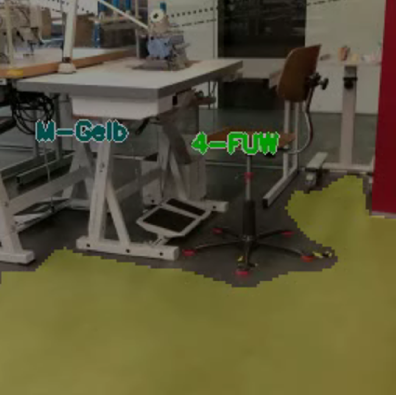
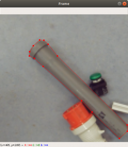
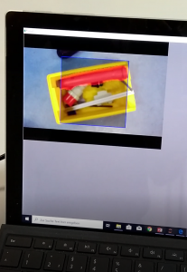
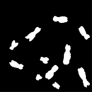
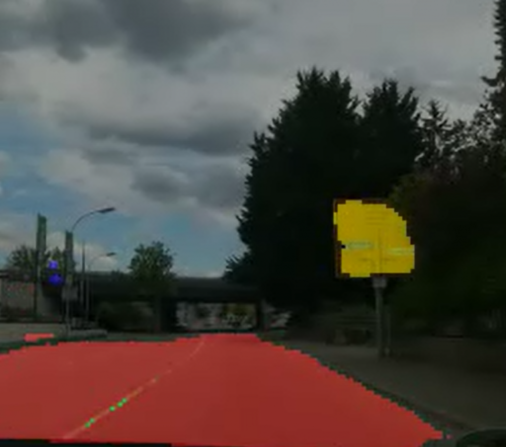
In Figure 5 you see a snapshot of the augmented video. The street is marked pretty well. You can even see how the sidewalk is not marked as a street. On the right side you find a traffic sign in yellow. The prediction works here good too. On the left side you find blue marking. The color blue categorizes cars. However there are no cars on the original image and therefore this is a misinterpretation. The street markings in green are not shown very well. In some parts of the augmented video they appear very strong, and in some parts you see only fragments, just like in Figure 5.

Figure 5: Snapshot of the augmented video

Overall we are very happy with the result of this project, considering that we have only labeled 250 images. We are convinced that we get better results as soon as we have more images for training. To overcome the problem we tried with data augmentation. So from the 250 images we created around 3000 images. We also randomly flipped the images horizontally in a code version, which was not discussed here.

We think that we have too much overfitting, which can only be solved with more training data. Due to the time limit, we had to restrict ourselves with fewer training data.

Acknowledgement

Special thanks to the class of Summer Semester 2020 Design Cyber Physical Systems providing the videos while driving and labeling the images for the training data used for the neural network. We appreciate this very much since this is a lot of effort.

Also special thanks to the University of Applied Science Albstadt-Sigmaringen for providing the infrastructure and the appliances to enable this class and this research.

Image Processing for an Autonomous Guided Vehicle in a Learn-Factory

In our school we are offering a master class for students from different faculties such as machine engineering, textile engineering and computer science. The content of the class involve modern topics in industry with practical work; the class is called Research Project Industry 4.0. During the summer semester 2020 we had 13 students enlisted, while most of them are textile engineers and few are computer scientists

The textile engineering faculty owns a room with different machines used for textile processing. They call this room learn-factory, see Figure 1. The intention is to show students how to process textile goods. Another intention is to produce textiles in small numbers ordered from industry.

Figure 1: Learn-factory

In Figure 1 you see stations consisting of stitching machines, sewing machines, cutters, ovens etc. Processing textile goods nowadays still have a lot hand crafting involved, however to stay competitive, we need a certain amount of automation to lower labor cost. The idea is to use an autonomous guided vehicle to transport pre-processed textile goods from one station to another. This would relieve the workers from leaving their station, so they can concentrate on their textile processing tasks.

We decided that the autonomous guided vehicle will orientate through the learn-factory with a simple camera system. Images from the camera system need to be segmented into parts, such as floor and machine stations. The floor segments of the images are important, so the vehicle knows where to drive, and the machine stations locations are important to find the destination. Segmenting images is a well known problem in machine learning (semantic segmentation) and can be addressed by using neural networks.

Preparation

In order to use a neural network to solve the segmentation problem, we need training data. Fortunately this time we have many students helping to create data. The first step is to create images from a perspective of an autonomous guided vehicle. The students mounted a smart phone on a trolley and took images while moving around the trolley, see Figure 2.

Figure 2: Smart Phone on Trolley

In Figure 3 you see the layout of the learn-factory created by the students. You see the floor in blue, and the stations with their names as white rectangle. The learn-factory was divided into parts from where the images have to be taken. Each part was assigned to one student.

Figure 3: Layout of Learn-Factory

We set the goal, that each student has to take 1000 images from different angles. With 13 participating students, we gathered 13000 images, which we assumed to be a good coverage of the complete learn-factory.

Creating Training Data

Figure 3 shows the layout of the learn-factory with 16 machine and working stations. They are categorized as “1-Nagel1”, “Tape1” etc. You find the complete list of categories in the python dictionary classes below. Also the floor (“Boden”) and the window (“Fenster”) have their assigned categories. Altogether there are 20. Numbers are assigned to each machine and working stations. The number 0 is a category which belongs to neither of the categories in the dictionary classes.

classes = {"1-Nadel1" : 1, 
          "1-Nadel2" : 2,
          "Tape1" : 3, 
          "Tape2" : 4, 
          "Boden" : 5, 
          "Tisch0" : 6,         
          "Tisch1" : 7,
          "Tisch2" : 8,
          "Tisch3" : 9,
          "Tisch4" : 10,
          "Tisch5" : 11,
          "M-blau" : 12,
          "M-Blau" : 12,          
          "M-gelb" : 13,
          "M-Gelb" : 13,
          "M-rot" : 14,
           "M-Rot" : 14,
          "4-FÃœW" : 15,
          "4-FUEW" : 15,
          "4-FÃœW" : 15,          
          "Fenster" : 16,
          "Ofen" : 17,   
          "Cutter" : 18,
          "Heizung" : 19,          
         }

As mentioned above every student created 1000 images from the learn-factory. The images need to be process further before training the neural network. We need to tell, which parts of the image belong to which category. See the categories in the code above.

The labelme website offers a downloadable tool to mask parts of the image and assign them to a label (or a category). Figure 4 shows a screenshot of the tool labelme. The student can create closed polygons by marking the vertices with a mouse click. Then the students assign a category to the polygon (Polygon Labels in Figure 4, right side).

Figure 4: Labelme

The tool labelme saves for each processed image a json file. The json file contains the list of polygons, described by their vertices, the names of the categories, and the image itself, which is saved as a base64 encoded image.

Figure 5: Creating Mask Images

The next step is to process the json files to extract the polygons and their names to create mask images, see Figure 5. On the left side of Figure 5 you see the tool labelme. In the middle you find a processed mask image, created by the polygons. On the right side there is an overlaid image from the original image and the mask image.

Data Processing

Each of the 13 students labeled 1000 images with the tool labelme. The tool labelme generates json files which can be parsed easily with python to extract the vertices of the labeled polygons. Each polygon is assigned to a category (this information can also be extracted from the json file) and each category is assigned a color. The python dictionary color in the code below shows the number/RGB-color assignment.

colors = {0 : (0,0,0), 
          1 : (0,0,55), 
          2 : (0,0,127),
          3 : (0,55,0), 
          4 : (0,127,0), 
          5 : (0,127,127), 
          6 : (40,0,0),         
          7 : (80,0,0),
          8 : (120,0,0),
          9 : (160,0,0),
          10 : (200,0,0),
          11 : (240,0,0),
          12 : (127,0,127),         
          13 : (127,127,0),
          14 : (0, 0, 255),
          15 : (0, 255 ,0),          
          16 : (0, 255 ,255),
          17 : (100, 0 ,0),   
          18 : (200,0,0),
          19 : (255,0,0),          
         }

dim = (128, 128) 

The function createMasks below is iterating through the list of json-files (13000 files!) located in sourcejsonsdir. In each iteration steps createMasks loads the content of the json file into data. It decodes the image tagged by imageData using the methods b64decode and imdecode and stores it into the variable img. The code verifies if the image is square and resizes it to 128×128.

Next, createMasks is iterating through all polygons in the json file, which are tagged as shapes. Again it iterates through all vertices of each shape and creates a polygon (rr and cc) from them. A mask image is created from the polygon and appended to a list of masks after it is resized to 128×128. The function createMasks sets the values of the pixels which are inside the polygon to the number which corresponds to the category:

mask_orig[rr,cc] = classes[shape[‘label’]]

Finally all masks are added to finalmask by using OpenCV’s threshold and bitwise_and operation. The function createMasks then stores the original image into destimagesdir and the mask image into destmasksdir.

def createMasks(sourcejsonsdir, destimagesdir, destmasksdir):

    assocf = open(os.path.join(path,"assoc_orig.txt"), "w")
    count = 0
    directory = sourcejsonsdir
    for filename in os.listdir(directory):
        if filename.endswith(".json"):
            print("{}:{}".format(count,os.path.join(directory, filename)))
            
            f = open(os.path.join(directory, filename))
            data = json.load(f)
            img_arr = data['imageData']  
            imgdata = base64.b64decode(img_arr)

            img = cv2.imdecode(np.frombuffer(imgdata, dtype=np.uint8), flags=cv2.IMREAD_COLOR)
   
            assert (img.shape[0] > dim[0])
            assert (img.shape[1] > dim[0])
           
            if img.shape[0] != img.shape[1]:
                print("shape is wrong: {},{} ... skipping".format(img.shape[0],img.shape[1]))
                continue

            img_resized = cv2.resize(img, dim, interpolation = cv2.INTER_NEAREST)

            finalmask = np.zeros((img_resized.shape[0], img_resized.shape[1]), 'uint8')
            mthresh = np.zeros((img_resized.shape[0], img_resized.shape[1]), 'uint8')
            masks=[]

            for shape in data['shapes']:
                assert(shape['label'] in classes)

                vertices = np.array([[point[1],point[0]] for point in shape['points']])
                vertices = vertices.astype(int)

                rr, cc = polygon(vertices[:,0], vertices[:,1], img.shape)
                mask_orig = np.zeros((img.shape[0], img.shape[1]), 'uint8')
                mask_orig[rr,cc] = classes[shape['label']]
                masks.append(cv2.resize(mask_orig, dim, interpolation = cv2.INTER_NEAREST))

            for m in masks:
                _,mthresh = cv2.threshold(m,1,255,cv2.THRESH_BINARY_INV)
                finalmask = cv2.bitwise_and(finalmask,finalmask,mask = mthresh)
                finalmask += m

            cv2.imwrite(os.path.join(destimagesdir, "{:05d}o.png".format(count)), img_resized)
            cv2.imwrite(os.path.join(destmasksdir, "{:05d}o.png".format(count)), finalmask)

            assocf.write("{:05d}o:{}\n".format(count, data['imagePath']))
            assocf.flush()
            count += 1

        else:
            continue
    f.close()

13000 mask images can now be used for training, just by processing the available data. However, we decided to generate more training data by using data augmentation. The function createMasksAugmented below works in a similar way as createMasks, therefore we just explain a few differences. The function createMasksAugmented rotates the original image with a random angle between -3 and 3 degrees and zooms into the rotated images with a random percentage (between 80 and 90 percent of the original image). The method imutils.rotate_bound is performing this operation. The final image is stored into image_zoomed. The mask image is generated the same way as in function createMasks. However createMasksAugmented rotates and zooms the mask image in the same way as the original image. More data augmentation is applied by OpenCV’s convertScaleAbs method. It modifies randomly contrast and brightness on the rotated and zoomed image before saving it into the destimagedir directory. The rotated and zoomed mask image is saved into the directory destmaskdir.

def createMasksAugmented(sourcejsonsdir, destimagesdir, destmasksdir):

    assocf = open(os.path.join(path,"assoc_augmented.txt"), "w")

    count = 0
    directory = sourcejsonsdir
    for filename in os.listdir(directory):
        if filename.endswith(".json"):
            print("{}:{}".format(count,os.path.join(directory, filename)))

            f = open(os.path.join(directory, filename))
            data = json.load(f)
            img_arr = data['imageData']  
            imgdata = base64.b64decode(img_arr)

            img = cv2.imdecode(np.frombuffer(imgdata, dtype=np.uint8), flags=cv2.IMREAD_COLOR)
            
            assert (img.shape[0] > dim[0])
            assert (img.shape[1] > dim[0])
            
            if img.shape[0] != img.shape[1]:
                print("shape is wrong: {},{} ... skipping".format(img.shape[0],img.shape[1]))
                continue
            
            zoom = randint(80,90)/100.0
            angle = (2*random()-1)*3.0
            img_rotated = imutils.rotate_bound(img, angle)
            
            xf = int(img_rotated.shape[0]*zoom)
            yf = int(img_rotated.shape[1]*zoom)            
            
            img_zoomed = np.zeros((xf, yf, img_rotated.shape[2]), 'uint8')
            img_zoomed[:,:,:] = img_rotated[int((img_rotated.shape[0]-xf)/2):int((img_rotated.shape[0]-xf)/2)+xf,int((img_rotated.shape[1]-yf)/2):int((img_rotated.shape[1]-yf)/2)+yf,:] 
            

            img_resized = cv2.resize(img_zoomed, dim, interpolation = cv2.INTER_NEAREST)

            finalmask = np.zeros((img_resized.shape[0], img_resized.shape[1]), 'uint8')
            mthresh = np.zeros((img_resized.shape[0], img_resized.shape[1]), 'uint8')
            masks=[]

            for shape in data['shapes']:
                assert(shape['label'] in classes)

                vertices = np.array([[point[1],point[0]] for point in shape['points']])
                vertices = vertices.astype(int)

                rr, cc = polygon(vertices[:,0], vertices[:,1], img.shape)
                mask_orig = np.zeros((img.shape[0], img.shape[1]), 'uint8')
                mask_orig[rr,cc] = classes[shape['label']]
                
                mask_rotated = imutils.rotate_bound(mask_orig, angle)
                
                mask_zoomed = np.zeros((xf, yf), 'uint8')
                mask_zoomed[:,:] = mask_rotated[int((img_rotated.shape[0]-xf)/2):int((img_rotated.shape[0]-xf)/2)+xf,int((img_rotated.shape[1]-yf)/2):int((img_rotated.shape[1]-yf)/2)+yf] 
                
                masks.append(cv2.resize(mask_zoomed, dim, interpolation = cv2.INTER_NEAREST))

            for m in masks:
                _,mthresh = cv2.threshold(m,1,255,cv2.THRESH_BINARY_INV)
                finalmask = cv2.bitwise_and(finalmask,finalmask,mask = mthresh)
                finalmask += m

            alpha = 0.8 + 0.4*random();
            beta = int(random()*15)
    
            img_adjusted = cv2.convertScaleAbs(img_resized, alpha=alpha, beta=beta)
        
            cv2.imwrite(os.path.join(destimagesdir, "{:05d}a.png".format(count)), img_adjusted)
            cv2.imwrite(os.path.join(destmasksdir, "{:05d}a.png".format(count)), finalmask) 

            assocf.write("{:05d}a:{}\n".format(count, data['imagePath']))
            assocf.flush()
            count += 1

        else:
            continue
    f.close()

The function createMasksAugmented was applied one time to all available data. So at the end we had 26000 images for training. Since createMasksAugmented uses random numbers for rotation, zooming, brightness and contrast, it could be applied even more than one time.

The UNET Model

We train our data on a UNET model, because we had good semantic segmentation results with this kind of model in previous projects. Hence, the neural network was already described in previous posts. Originally we took the code from here, however modified it slightly to match our purpose. The first function is conv2d_block which executes two convolutions and relu-activation operations in a row, see code below.

def conv2d_block(input_tensor, n_filters, kernel_size=3, batchnorm=True):
    # first layer
    x = Conv2D(filters=n_filters, kernel_size=(kernel_size, kernel_size), kernel_initializer="he_normal",
               padding="same")(input_tensor)
    if batchnorm:
        x = BatchNormalization()(x)
    x = Activation("relu")(x)
    # second layer
    x = Conv2D(filters=n_filters, kernel_size=(kernel_size, kernel_size), kernel_initializer="he_normal",
               padding="same")(x)
    if batchnorm:
        x = BatchNormalization()(x)
    x = Activation("relu")(x)
    return x

The code get_unet below builds up the model by calling conv2_block and maxpooling2D several times (this is called the contracting path). The output of maxpooling2D operations are stored in variables (c1, c2, c3, c4) which are fed later into the expansive path. At the expansive path, get_unet calls reverse convolution operations and concatenates the saved variables (c1, c2, c3, c4) from the contracting path with the output of the Conv2DTranspose operations. In the line:

c10 = Conv2D(len(colors), (1, 1), activation=”softmax”) (c9)

you find the minor change we made. The output size of the model will be an image of size 128×128 with 20 (which is len(color)) layers.

def get_unet(input_img, n_filters=16, dropout=0.5, batchnorm=True):
    # contracting path
    c1 = conv2d_block(input_img, n_filters=n_filters*1, kernel_size=3, batchnorm=batchnorm)
    p1 = MaxPooling2D((2, 2)) (c1)
    p1 = Dropout(dropout*0.5)(p1)

    c2 = conv2d_block(p1, n_filters=n_filters*2, kernel_size=3, batchnorm=batchnorm)
    p2 = MaxPooling2D((2, 2)) (c2)
    p2 = Dropout(dropout)(p2)

    c3 = conv2d_block(p2, n_filters=n_filters*4, kernel_size=3, batchnorm=batchnorm)
    p3 = MaxPooling2D((2, 2)) (c3)
    p3 = Dropout(dropout)(p3)

    c4 = conv2d_block(p3, n_filters=n_filters*8, kernel_size=3, batchnorm=batchnorm)
    p4 = MaxPooling2D(pool_size=(2, 2)) (c4)
    p4 = Dropout(dropout)(p4)
    
    c5 = conv2d_block(p4, n_filters=n_filters*16, kernel_size=3, batchnorm=batchnorm)
    
    # expansive path
    u6 = Conv2DTranspose(n_filters*8, (3, 3), strides=(2, 2), padding='same') (c5)
    u6 = concatenate([u6, c4])
    u6 = Dropout(dropout)(u6)
    c6 = conv2d_block(u6, n_filters=n_filters*8, kernel_size=3, batchnorm=batchnorm)

    u7 = Conv2DTranspose(n_filters*4, (3, 3), strides=(2, 2), padding='same') (c6)
    u7 = concatenate([u7, c3])
    u7 = Dropout(dropout)(u7)
    c7 = conv2d_block(u7, n_filters=n_filters*4, kernel_size=3, batchnorm=batchnorm)

    u8 = Conv2DTranspose(n_filters*2, (3, 3), strides=(2, 2), padding='same') (c7)
    u8 = concatenate([u8, c2])
    u8 = Dropout(dropout)(u8)
    c8 = conv2d_block(u8, n_filters=n_filters*2, kernel_size=3, batchnorm=batchnorm)

    u9 = Conv2DTranspose(n_filters*1, (3, 3), strides=(2, 2), padding='same') (c8)
    u9 = concatenate([u9, c1], axis=3)
    u9 = Dropout(dropout)(u9)
    c9 = conv2d_block(u9, n_filters=n_filters*1, kernel_size=3, batchnorm=batchnorm)
    
    c10 = Conv2D(len(colors), (1, 1), activation="softmax") (c9)
   
    model = Model(inputs=[input_img], outputs=[c10])
    return model

We mentioned above that we created mask images from the json files, which have a size of 128×128. Each category is simply assigned a number between 0 and 19 at each pixel position. However the neural network has an output of 128x128x20. We use for the neural network a different mask representation, because this way it is preferred for training. Hence, each layer of the 128x128x20 image gets its own category assigned. If a pixel of an image layer is one, it marks the position of an object with its category; if the pixel is zero, it marks that no object of the former category is at this position. Since this is a preferred representation for neural networks, we need to convert the 128×128 masks (created from json files) to 128x128x20 masks. The function makecolormask below is performing this operation. Note that there are more efficient ways to convert the masks, but this will be discussed in a later post.

def makecolormask(mask):
    ret_mask = np.zeros((mask.shape[0], mask.shape[1], len(colors)), 'uint8')
    for i in range(mask.shape[0]):
        for j in range(mask.shape[1]):
                assert(mask[i,j] < len(colors))
                ret_mask[i,j,mask[i,j]] = 1
    return ret_mask

In this project we ran into a problem, which we have not seen in previous projects yet. As mentioned above, we generated 26000 original images and 26000 mask images. Loading all images into memory and with a 8GB NVIDIA graphic card will break the training. Therefore we created the function generatebatchdata to load original and mask images in smaller batches into memory, see code below. The parameters of the functions are fullpathimages and fullpatchmasks which point to the directories of the training data. The lists imagenames and masknames contain the filenames of the original and mask images.

The function generatebatchdata reads the data in (cv2.imread) and appends the data to imagelist and masklist. Here the makecolormask function is applied to convert the json mask image to a 128x128x20 representation. The original images are processed even further with a mean and a standard deviation operations for normalization. Finally the imagelist and masklist is returned with the yield function. Obviously generatebatchdata is executed concurrently. The yield function stops the execution, until the training process continues to execute generatebatchdata with the next batch.

def generatebatchdata(batchsize, fullpathimages, fullpathmasks, imagenames, masknames):
  
    assert(len(imagenames) == len(masknames))

    while True:
        batchstart = 0
        batchend = batchsize    
        
        while batchstart < len(imagenames):
            
            imagelist = []
            masklist = []
            
            limit = min(batchend, len(imagenames))

            for i in range(batchstart, limit):
                if imagenames[i].endswith(".png"):
                    imagelist.append(cv2.imread(os.path.join(fullpathimages,imagenames[i]),cv2.IMREAD_COLOR ))
                if masknames[i].endswith(".png"):
                    masklist.append(makecolormask(cv2.imread(os.path.join(fullpathmasks,masknames[i]),cv2.IMREAD_UNCHANGED )))


            train_data = np.array(imagelist, dtype=np.float32)
            train_mask= np.array(masklist, dtype=np.float32)

            train_data -= train_data.mean()
            train_data /= train_data.std()
    
            yield (train_data,train_mask)    

            batchstart += batchsize   
            batchend += batchsize

In the code below you see that the function generatebatchdata is instantiated twice. One time for training data, and one time for validation data. Previously we selected randomly about 15% of the original and mask images and moved them to validation directories (fullpathimagesvalid and fullpathmasksvalid).

generator_train = generatebatchdata(30, fullpathimages, fullpathmasks, imagenames, masknames)
generator_valid = generatebatchdata(30, fullpathimagesvalid, fullpathmasksvalid,  imagenamesvalid, masknamesvalid)

The UNET model is instantiated and compiled in the code below. As input the model expects images with dimension dim with three layers (RGB) which is 128x128x3.

input_img = Input((dim[0], dim[1], 3), name='img')
model = get_unet(input_img, n_filters=len(colors), dropout=0.05, batchnorm=True)
model.compile(optimizer=Adam(), loss="categorical_crossentropy", metrics=["accuracy"])

During training we use three callback function. The first callback is EarlyStopping, which stops the training process if there is no improvement of the loss value after ten epochs. The next callback ReduceLROnPlateau modifies the learning rate if there is no imrovement concerning loss after three epochs. The last callback ModelCheckpoint saves a checkpoint of the model during the training process if the model has improved its loss value.

callbacks = [
    EarlyStopping(patience=10, verbose=1),
    ReduceLROnPlateau(factor=0.1, patience=3, min_lr=0.00001, verbose=1),
    ModelCheckpoint(os.path.join(path, dirmodels,"model-chkpt.h5"), verbose=1, save_best_only=True, save_weights_only=True)
]

Below the code starts the training process. The training was executed on a NVIDIA 2070 graphic card with 8GB memory. It turned out that we have a accuracy of 95,3% and a validation accuracy of 94,9%. So we have a small overfitting. Training time was about 20 minutes.

model.fit_generator(generator_train,steps_per_epoch=530, epochs=20, callbacks=callbacks, validation_data=generator_valid, validation_steps=3064)

The function predictedmask below is a utility function to create mask images from the model’s output back to the original mask image form we received after processing the json files. It is a reverse function of makecolormask. The function predictedmask is useful to create masks as seen as in Figure 6 (in the middle) for display purpose. Since 128x128x20 images cannot be displayed in such a way.

def predictedmask(masklist):
    y_list = []
    for mask in masklist:
        assert mask.shape == (dim[0], dim[1], 20)
        imgret = np.zeros((dim[0], dim[1]), np.uint8)
        for i in range(dim[0]):
            for j in range(dim[1]):
                result = np.where(mask[i,j,:] == np.amax(mask[i,j,:]))
                assert result[0][0] < len(colors)
                imgret[i,j] = result[0][0]
        y_list.append(imgret)
    return y_list

Figure 6 shows a verification example. An original image (left) was put into the trained model with the model’s predict method (model.predict) and the result can be seen in Figure 6 in the middle. The function predictedmask was applied here. Overlaying the left and the middle image results to the right image.

Figure 6: Verifying the model

Creating an augmented video

The goal of this project is to create an augmented life video from the learn-factory while walking through with a video camera. The application should mask the floor, and the machines should be labeled with text, which are the categories. Basically each image of the video is fed into the trained neural network and it predicts a 128x128x20 mask image. However, further processing is needed, such as labeling the video images with text.

The function predictedmask above converts 128x128x20 mask images back to 128×128 mask images. The pixel values are values between 0 and 19. The python dictionary categories below shows an assignment between the values and the categories written as text. A similar assignment (python dictionary classes) we have above, but here it is just the way around.

categories = {1: "1-Nadel1", 
              2: "1-Nadel2",
              3: "Tape1", 
              4: "Tape2", 
              5: "Boden", 
              6: "Tisch0",         
              7: "Tisch1",
              8: "Tisch2",
              9: "Tisch3",
              10: "Tisch4",
              11: "Tisch5",
              12: "M-Blau",          
              13: "M-Gelb",
              14: "M-Rot",
              15: "4-FUW",          
              17: "Ofen",   
              18: "Cutter",
              19: "Heizung",          
         }

As already mentioned, the masks created by predictedmask are one layer images, whose pixels values are between 0 and 19. In order to convert the masks to a color image the function makemaskcolor is used. It uses the python dictionary colors to assign each pixel value to a color value. The output of makemaskcolor is a colored mask image of one category with shape 128x128x3. The parameter color indicates from which category a mask should be created. Such as, if you want the mask of a floor (Boden, see python dictionary categories), the value of color should be five. In a later post, we can show how this operation can be done more efficient.

def makemaskcolor(mask, color):
    ret_mask = np.zeros((mask.shape[0], mask.shape[1], 3), 'uint8')
    for i in range(mask.shape[0]):
        for j in range(mask.shape[1]):
                if mask[i,j] == color:
                    ret_mask[i,j,0] = colors[color][0]
                    ret_mask[i,j,1] = colors[color][1]
                    ret_mask[i,j,2] = colors[color][2]
    return ret_mask

Below the code of the function markpicture. The input parameter inp_img is a mask image from the predictedmask ouput. The parameter orig_img is the original image, which has been fed into the neural network model for the mask prediction. We decided to show only the mask of the floor. The function markpicture creates with the following code the floor mask (boden stands for floor):

boden = makemaskcolor(inp_img,5)

Then the function markpicture iterates through the category values, however it omits 5 and 16. The category 16 is a window (Fenster stands for window) and needs no label. OpenCV’s inRange Method extracts the i’th mask (see for loop) and assigns it to inp_img_new. The code calls OpenCV’s findContour to get the contour of the i’th category. The contour needs to exceed a minimum area, which can be determined by cv2.contourArea. The code then calculates the center of gravity of the contour and puts text indicating the category at this position onto the original image. Text is put two times there; first white text with a larger boldness and second text in color of the category (see dictionary color) and a smaller boldness. By doing this, we improve to emphasize the text on the image. Finally markpicture overlays the processed image with the floor (cv2.addWeighted) and returns the image.

def markpicture(inp_img, orig_img):

    update_img = orig_img.copy()

    img_new = np.zeros((inp_img.shape[0], inp_img.shape[1],3), 'uint8')
    inp_img_new = np.zeros((inp_img.shape[0], inp_img.shape[1],3), 'uint8')
    boden = np.zeros((inp_img.shape[0], inp_img.shape[1],3), 'uint8')
    boden_resized = np.zeros((orig_img.shape[0], orig_img.shape[1],3), 'uint8')
    weighted = np.zeros((orig_img.shape[0], orig_img.shape[1],3), 'uint8')

    boden = makemaskcolor(inp_img,5)

    for i in [1,2,3,4,6,7,8,9,10,11,12,13,14,15,17,18,19]:

        inp_img_new = inp_img.copy()
        inp_img_new = inp_img_new.astype(np.uint8)

        inp_img_new = cv2.inRange(inp_img_new,i,i)
        contours,_ = cv2.findContours(inp_img_new,cv2.RETR_TREE,cv2.CHAIN_APPROX_NONE)

        if len(contours) > 0:

            contours = sorted(contours, key=cv2.contourArea,  reverse=True)

            M = cv2.moments(contours[0])
            area = cv2.contourArea(contours[0])
            if M['m00'] > 0 and area > 600:
                
                cx = int(int(M['m10']/M['m00'])*orig_img.shape[0]/inp_img.shape[0])
                cy = int(int(M['m01']/M['m00'])*orig_img.shape[1]/inp_img.shape[1])
                update_img= cv2.putText(update_img,categories[i],(cx,cy), cv2.FONT_HERSHEY_SIMPLEX,0.5 if area > 800 else 0.25, (255,255,255), 4) 
                update_img= cv2.putText(update_img,categories[i],(cx,cy), cv2.FONT_HERSHEY_SIMPLEX,0.5 if area > 800 else 0.25, colors[i], 2 if area > 500 else 1) 
            
    boden_resized = cv2.resize(boden, (orig_img.shape[0], orig_img.shape[1]), interpolation = cv2.INTER_AREA) 

    assert(boden_resized.shape == update_img.shape)
    cv2.addWeighted(update_img, 0.6, boden_resized, 0.4, 0, weighted)            
            
    return weighted

In Figure 7 you can find an output of maskpicture. On the left side a representation of the mask from the neural network prediction and on the right side a processed original image with text and overlaid floor. You find here the text of the categories Tape1 and Tape2.

Figure 7: Mask and labeled original image

To create an augmented video we used the code below. Before augmentation we walked through the learn-factory and created a normal video from a robot’s perspective and named it video.mp4. OpenCV’s VideoCapture opens the video and iterates through it image by image. VideoCaputure’s read method extracts each image from the video and assigns it to frame. frame is resized and normalized. Then the code feeds it into the neural network’s predict method. The output is a predicted mask (with shape 128x128x20), which is converted to another mask representation with the function predictedmask (shape 128×128). Its output is fed into markpicture, which is putting text on the image and marking the floor. Finally the image is written to a new video videounet128-1.mp4.

cap = cv2.VideoCapture(os.path.join(path,"videos",'video.mp4'))
if (cap.isOpened() == True): 
    
    print("Opening video stream or file")
    out = cv2.VideoWriter(os.path.join(path,"videos",'videounet128-1.mp4'),cv2.VideoWriter_fourcc(*'MP4V'), 25, (256,256))
    while(cap.isOpened()):
        ret, frame = cap.read()
        
        if ret == False:
            break
        
        frame_resized = np.zeros((dim[0], dim[1], 3), 'uint8')  
        frame_resized = cv2.resize(frame, (dim[0],dim[1]), interpolation = cv2.INTER_AREA) 
        test_data = []
        test_data.append(frame_resized)
        test_data = np.array(test_data, dtype=np.float32)
        test_data -= test_data.mean()
        test_data /= test_data.std()
        
        predicted = model.predict(test_data, batch_size=1, verbose=0)
        assert(len(predicted) == 1)
        pmask = predictedmask(predicted[0])
        
        if ret == True:
            img = markpicture(pmask, frame)
            out.write(img)
            cv2.imshow('Frame',img)
            if cv2.waitKey(25) & 0xFF == ord('q'):
                break

    out.release()
            
cap.release()
cv2.destroyAllWindows()

Conclusion

The resulting videos are astonishing. You can walk through the learn-factory with a video camera and process in real-time the video and you receive an output such as displayed in Figure 8. The machines are mostly labeled correctly and the floor indicates where a autonomous guided vehicle could drive.

Figure 8: Snapshot of an augmented video

There are situations where the labeling works not correctly, especially if you walk into areas, where the students have not taken any pictures and therefore no labeling was done. In Figure 3 it is the area on the right side. Figure 9 shows such a snapshot where the labeling is completely incorrect. However the floor is still predicted correctly. Note that no training data existed for this area, so the chaotic prediction is expected.

Figure 9: Snapshot of video with chaotic predictions

Acknowledgement

Special thanks to the class of Summer Semester 2020 Forschungsprojekt Industrie 4.0 providing the images of the learn-factory (13000!) and labeling the images for the training data (also 13000!!) used for the neural network. We appreciate this very much, and we know how much effort you have put into this.

Also special thanks to the University of Applied Science Albstadt-Sigmaringen for hosting the learn-factory and providing the appliances to enable this research.

Centromere Position on a Chromosome Image using a Neural Network

Chromosomes have one short arm and one long arm. The centromere sits in between and links both arms together. Biologists find it convenient that an application can spot automatically the position of the centromere on a chromosome image. In general for image processing, it is useful for an application to know the centromere position to simplify the classification of the chromosome type.

With this project we want to show how an application can get the centromere positions by using a neuronal network. In order to train the neuronal network, we need sufficient training data. We show here, how we created the training data. A position in an image is a coordinate with two numbers. The application must therefore use an neuronal network with an regression layer as an output. In this post we show what kind of neuronal network we used for retrieving a position from an image.

Creating the Training Data

Previously we created with a tool around 3000 images from several complete chromosome images. We do not go much into detail about this tool. The tool works in a way that it loads in and shows a complete chromosome image with its 46 chromosomes and as an user we can select with the mouse a square on this image. The content of the square is then saved as a 128×128 chromosome image and as a 128×128 telomere image. Figure 1 shows an example of both images. We have created around 3000 chromosome and telomere images from different positions.

Figure 1: Chromosome Image and Telomere Image

Each time we save the chromosome and telomere images, the application updates a csv file with the name of the chromosome (chrname) and the name of the telomere (telname) using the write function of the code below. It uses the library pandas to concat rows to the end of a csv file with the name f_name.

def write(chrname, telname, x, y): 
  
    if isfile(f_name): 
  
        df = pd.read_csv(f_name, index_col = 0) 
        data = [{'chr': chrname, 'tel': telname, 'x': x, 'y':y}] 
        latest = pd.DataFrame(data) 
        df = pd.concat((df, latest), ignore_index = True, sort = False) 
    else: 
        data = [{'chr': chrname, 'tel': telname, 'x': x, 'y':y}] 
        df = pd.DataFrame(data) 

    df.to_csv(f_name) 

In the code above, you can see that a x and a y value is stored into the csv file, as well. This is the position of the centromere of the chromosome on the chromosome image. At this point of time, the position is not known yet. We need a tool, where we can click on each image to mark the centromere position. The code of the tool is shown below. There are two parts. The first part is the callback function click. It is called as soon as the user of the application presses a mouse button or moves the mouse. If the left mouse button is pressed, then the actual mouse position on the conc window is moved to the variable refPt. The second part of the tool loads in the a chromosome image from a directory chrdestpath and a telomere image from a directory teldestpath into a window named conc. The function makecolor (this function is described below) adds both images together to one image. The user can select with the mouse the centromere position and a cross appears on the clicking position, Figure 2. The application stores the position refPt by pressing the key “s” into the pandas data frame df. After this, the application loads in the next chromosome image from the directory chrdestpath and the next telomere image from the directory teldestpath.

refPt = (0,0)
mouseevent = False
def click(event,x,y,flags,param):
    global refPt
    global mouseevent
    if event == cv2.EVENT_LBUTTONDOWN:
        refPt = (x,y)
        mouseevent = True

cv2.namedWindow('conc')
cv2.setMouseCallback("conc", click)

theEnd = False
theNext = False

img_i=0
imgstart = 0
assert imgstart < imgcount

df = pd.read_csv(f_name, index_col = 0) 

for index, row in df.iterrows():
 
    if img_i < imgstart:
        img_i = img_i + 1
        continue
        
    chrtest = cv2.imread("{}{}".format(chrdestpath,row["chr"]),1)
    teltest = cv2.imread("{}{}".format(teldestpath,row["tel"]),1)
    
    conc = makecolor(chrtest, teltest)
    concresized = np.zeros((conc.shape[0]*2, conc.shape[1]*2,3), np.uint8)
    concresized = cv2.resize(conc, (conc.shape[0]*2,conc.shape[1]*2), interpolation = cv2.INTER_AREA)
    
    refPt = (row["y"],row["x"])
    cv2.putText(concresized,row["chr"], (2,12), cv2.FONT_HERSHEY_SIMPLEX, 0.4, (0, 255, 0), 1, cv2.LINE_AA)

    while True:
        cv2.imshow('conc',concresized)
        key = cv2.waitKey(1)
        if mouseevent == True:
            print(refPt[0], refPt[1])
            concresized = cross(concresized, refPt[0], refPt[1], (255,255,255))
            mouseevent = False
        if key & 0xFF == ord("q") :
            theEnd = True
            break
        if key & 0xFF == ord("s") :
            df.loc[df["chr"] == row["chr"], "x"] = refPt[1]//2
            df.loc[df["chr"] == row["chr"], "y"] = refPt[0]//2
            theNext = True
            break
        if key & 0xFF == ord("n") :
            theNext = True
            break
    if theEnd == True:
        break
    if theNext == True:
        theNext = False
           
df.to_csv(f_name) 
cv2.destroyAllWindows()

Figure 2 shows the cross added to the centromere position selected by the user. This procedure was done around 3000 times on chromosome and telomere images, so the output was a csv file with 3000 chromosome image names, telomere image names, and centromere positions.

Figure 2: Centromere Postion on a Chromosome Image

Augmenting the Data

In general 3000 images are too few images to train a neuronal network, so we augmented the images to have more training data. This was done by mirrowing all chromosome images (and its centromere positions) on the horizontal axis and on the vertical axis. This increased the number of images to 12000. The code below shows the load_data function to load the training data or validation_data into arrays

def load_data(csvname, chrdatapathname, teldatapathname):
    X_train = []
    y_train = []
    
    assert isfile(csvname) == True
    df = pd.read_csv(csvname, index_col = 0) 
    for index, row in df.iterrows():
                          
        chrname = "{}{}".format(chrdatapathname,row["chr"])
        telname = "{}{}".format(teldatapathname,row["tel"])
    
        chrimg = cv2.imread(chrname,1)
        telimg = cv2.imread(telname,1)                  
                 
        X_train.append(makecolor(chrimg, telimg))
        y_train.append((row['x'],row['y']))
    return X_train, y_train

In the code above you find a makecolor function. makecolor copies the grayscale images of the chromosome into the green layer of a new color image and the telomere image into the red layer of the same color image, see code of the function makecolor below.

def makecolor(chromo, telo):

    chromogray = cv2.cvtColor(chromo, cv2.COLOR_BGR2GRAY)
    telogray = cv2.cvtColor(telo, cv2.COLOR_BGR2GRAY)
    
    imgret = np.zeros((imgsize, imgsize,3), np.uint8)
    
    imgret[0:imgsize, 0:imgsize,1] = chromogray
    imgret[0:imgsize, 0:imgsize,0] = telogray
    
    return imgret

Below the function code mirrowdata to flip the images horizontally or vertically. It uses the parameter flip to control the flipping of the image and its centromere position.

 def mirrowdata(data, target, flip=0): 
    xdata = []
    ytarget = []

    for picture in data:
        xdata.append(cv2.flip(picture, flip))
        
    for point in target:
        if flip == 0:
            ytarget.append((imgsize-point[0],point[1]))
        if flip == 1:
            ytarget.append((point[0],imgsize-point[1]))
        if flip == -1:
            ytarget.append((imgsize-point[0],imgsize-point[1]))
    
    return  xdata, ytarget

The following code loads in the training data into the array train_data and the array train_target. train_data contains color images of the chromosomes and telomeres and train_target contains the centromere positions. The mirrowdata function is applied twice on the data with different flip parameter settings. After this, the data is converted to numpy arrays. This needs to be done to be able to normalize the images with the mean function and the standard deviation function. This is done for 10000 images among the 12000 images for the training data. The same is done with the remaining 2000 images for the validation data.

train_data, train_target = load_data(csvtrainname, chrtrainpath, teltrainpath)
train_mirrow_data, train_mirrow_target = mirrowdata(train_data, train_target, 0)
train_data = train_data + train_mirrow_data
train_target = train_target + train_mirrow_target
train_mirrow_data, train_mirrow_target = mirrowdata(train_data, train_target, 1)
train_data = train_data + train_mirrow_data
train_target = train_target + train_mirrow_target

train_data = np.array(train_data, dtype=np.float32)
train_target = np.array(train_target, dtype=np.float32)

train_data -= train_data.mean()
train_data /= train_data.std()

Modeling and Training the Neuronal Network

Since we have images we want to feed into the neural network, we decided to use a neuronal network with convolution layers. We started with a Layer having 32 filters. As input for training data we need images with size imgsize, which is in our case 128. After each convolution layer we added the max pooling function with pool_size=(2,2) which reduces the size of the input data by half. The output is fed into the next layer. Altogether we have four convolution layers. The number of filters, we increase after each layer. After the fourth layer we flatten the network and feed this into the first dense layer. Then we feed the output into the second dense layer having only two neurons. The activation function is a linear function. This means, we will receive two float values, which is supposed to be the position of the centromere. As a loss function we decided to use the mean_absolute_percentage_error.

model = Sequential()
model.add(Conv2D(32, (3, 3), activation='relu', kernel_initializer='he_uniform', kernel_regularizer=l2(0.01), bias_regularizer=l2(0.01), padding='same', input_shape=(imgsize, imgsize, 3)))
model.add(MaxPooling2D((2, 2)))
model.add(Conv2D(32, (3, 3), activation='relu', kernel_initializer='he_uniform', kernel_regularizer=l2(0.01), bias_regularizer=l2(0.01), padding='same'))
model.add(MaxPooling2D((2, 2)))
model.add(Conv2D(64, (3, 3), activation='relu', kernel_initializer='he_uniform', kernel_regularizer=l2(0.01), bias_regularizer=l2(0.01), padding='same'))
model.add(MaxPooling2D((2, 2)))
model.add(Conv2D(128, (3, 3), activation='relu', kernel_initializer='he_uniform', kernel_regularizer=l2(0.01), bias_regularizer=l2(0.01), padding='same'))
model.add(MaxPooling2D((2, 2)))
model.add(Flatten())
model.add(Dense(128, activation='relu', kernel_initializer='he_uniform'))
model.add(Dropout(0.1))
model.add(Dense(2, activation='linear'))
opt = Adam(lr=1e-3, decay=1e-3 / 200)
model.compile(loss="mean_absolute_percentage_error", optimizer=opt, metrics=['accuracy'])

We start the training with the fit method. The input parameters are the list of colored and normalized chromosome images (train_data), the list of centromere positions (train_target), and the validation data (valid_data, valid_target). A callback function was defined to stop the training as soon as there is no progress seen. Also checkpoints are saved automatically, e.g. if there is progress during the training.

callbacks = [
    EarlyStopping(patience=10, verbose=1),
    ReduceLROnPlateau(factor=0.1, patience=3, min_lr=0.00001, verbose=1),
    ModelCheckpoint('modelregr.h5', verbose=1, save_best_only=True, save_weights_only=True)
]

model.fit(train_data, train_target, batch_size=20, nb_epoch=50, callbacks=callbacks, verbose=1, validation_data=(valid_data, valid_target) )

The training took around five minutes on a NVIDIA 2070 graphics card. The accuracy is 0.9462 and the validation accuracy is 0.9258. This shows a small overfitting. The loss function shows the same overfitting result.

Testing

We kept a few chromosome images and telomere images aside for testing and predicting. The images were stored in a test_data array and normalized before prediction. The prediction was done with the following code.

predictions_test = model.predict(test_data, batch_size=50, verbose=1)

prediction_test contains now all predicted centromere positions. Figure 3 shows the positions added to the chromosome images. We can see that the position of the cross is pretty close to the centromere. However there are deviations.

Figure 3: Predicted centromere positions

For displaying the chromosomes as shown as in Figure 3 we use the following showpics function. Note in case you want to use this code, you have to be aware that the input images may not be normalized, otherwise you see see a black image.

def showpics(data, target, firstpics=0, lastpics=8):
    chrtail=[]
    pnttail=[]
    columns = 4
    print(data[0].shape)
    for i in range(firstpics, lastpics):
        chrtail.append(data[i])
        pnttail.append(target[i])
    rows = (lastpics-firstpics)//columns
    fig=figure(figsize=(16, 4*rows))
    for i in range(columns*rows):
        point = pnttail[i]
        fig.add_subplot(rows, columns, i+1)
        pic = np.zeros((chrtail[i].shape[0], chrtail[i].shape[1],3), np.uint8)
        pic[0:pic.shape[0], 0:pic.shape[1], 0] = chrtail[i][0:pic.shape[0], 0:pic.shape[1], 0]
        pic[0:pic.shape[0], 0:pic.shape[1], 1] = chrtail[i][0:pic.shape[0], 0:pic.shape[1], 1]
        pic[0:pic.shape[0], 0:pic.shape[1], 2] = chrtail[i][0:pic.shape[0], 0:pic.shape[1], 2]
        imshow(cross(pic, int(point[1]), int(point[0]), (255,255,255)))    

Conclusion

The intention of this project was to show how to use linear regression as the last layer of the neuronal network. We wanted to get a position (coordinates) from an image.

Firstly we marked about 3000 centromere positions of chromosomes and telomere images with a tool we created. Then we augmented the data to increase the data to 12000 images. We augmented the data by horizontal and vertical flipping.

Secondly we trained a multilayer convolutional neural network with four convolutional layers and two dense layers. The last dense layer has two neurons. One for each coordinate.

The prediction result was fairly good, considering the little effort we used to optimize the model. On Figure 3 we still can see that the centromere position is not always hit on the right spot. We expect improvement after we will add more data and optimize the model.

PVC Pipe Recognition in Trash with Machine Learning

Introduction

The major work for recycling companies consist of sorting trash before processing it further. Usually recyclable trash is delivered in containers and employees in excavators sort out the parts such as electronics, metals, plastics etc. before moving them onto assembly lines. The assembly lines have additional sensors and machinery to sort the trash even further until it is finally shredded. The shredded trash is very often used as an energy source in the concrete industry.

Due to law regulations, there is a limit of chlorine substance inside burnable energy source. Since many plastics consist of polyvinyl chloride (PVC), which contains chlorine, the recycling company must take a lot of effort to sort out PVC from the trash in order to sell the shredded trash as an burnable energy source.

The idea of this project is to create an application, which takes life images from the content of a container and highlights the pieces of PVC trash on a monitor or on augmentation glasses worn by the employee. So the employee in the excavator gets help from the application, which is showing which pieces he has to sort out with his excavator, before moving the trash onto the assembly lines.

We introduce an application, which will use machine learning methods for highlighting the PVC trash pieces. Since objects from PVC can have many sizes and forms, we will limit our application in recognizing PVC pipes having gray color. Figure 1 is showing such a pipe. The application should highlight each pixel containing the PVC pipe with color, so it stands out of the picture.

Figure 1: PVC pipe

Segmenting PVC Pipe Regions using U-Net

Since the application is marking segments from the image, we are facing a segmentation problem. Segmentation problems are very often solved in machine learning with U-Nets. A description of U-Nets can be found here. Our description of the same U-Net, which is used in this work, can be found here.

So the application needs firstly to take real life images from a camera with scenes of trash, secondly to process the images with a trained U-Net model to receive the regions with PVC pipes and then thirdly to add the output image of the U-Net model with the original image. The output image is then displayed to the employee e.g. on a display. In Figure 2 you can see such a scene containing a PVC pipe.

Figure 2: Scene of trash

The items seen in Figure 2 will be used for training the U-Net model. So the next step is to generate many images of different configurations of item positions and light conditions for the model training.

There are two kind of images need to be fed into the U-Net model: the original image and the image containing a mask of the PVC pipe, indicating which pixel is a pipe, and which is not a pipe. We have therefore for each pixel two categories: pipe or not a pipe. So not only we need many original images but also we need many corresponding mask images. The mask images must be processed from the original images. In Figure 3 you can see what needs to be fed into the U-Net model for training, but the number of different kinds a images with different configurations needs to be in the thousands to get good results. The pixels of the mask image (right) in Figure 3 indicates if the pixel of the left image is a PVC pipe (white pixel) or not a PVC pipe (black pixel).

Figure 3: Original and mask image

Generating the training data set

I mentioned before that we need thousands of original and mask training images to get good results with training the model and with predicting the mask image from the trained model. In order to receive so many images, we need a strategy to create such a large number of images. Photographing thousands of scenes is possible, but very tedious. In order to receive the masks from the original image we need an ergonomic tool to create the masks in a very easy and fast way. Another strategy to improve the effort for gathering images is using an augmentation tool.

In this project, we programmed a tool, where the user can select the outline of the PVC pipe by clicking points on the original image. A polygon is create from the sequence of points, which is fed into the OpenCV function fillPoly to create the mask. Part of the source code is shown below:

pathnameimages = "/home/inf/Daten/Trash/images2/"
pathnamecuts = "/home/inf/Daten/Trash/train3/cuts/"
pathnamemasks = "/home/inf/Daten/Trash/train3/masks/"

def mouse_drawing(event, x, y, flags, params):
    global polygon
    global clicked
    if event == cv2.EVENT_LBUTTONDOWN:
        print("Left click:({},{})".format(x, y))
        polygon.append((x, y))
        clicked = True

dirlist = os.listdir(pathnameimages)

dirlist.sort()

fromto = (0,len(dirlist))

for i in range(fromto[0], fromto[1]):

    if stop == True:
        break
    print(dirlist[i])

    img = join(pathnameimages, dirlist[i])
    file = cv2.imread(img, 1)
    assert file.shape[0] == file.shape[1]
    img = np.zeros([file.shape[0]*2, file.shape[1]*2,3], dtype=np.uint8)       
    img = cv2.resize(file.copy(), (incshape[0], incshape[1]), interpolation = cv2.INTER_AREA) 
                    
    original = img.copy()

    polygon.clear()

    cv2.namedWindow("Frame")
    cv2.setMouseCallback("Frame", mouse_drawing)

    while True:
        
        cv2.imshow("Frame", img)
        key = cv2.waitKey(1)

        if key & 0xFF == ord("n"):
            break
                    
        if key & 0xFF == ord("q"):
            stop = True
            break                    
                    
        if key & 0xFF == ord("c") and len(polygon) > 0:
            cnt = np.array(polygon)
            mask = np.zeros(original.shape, dtype=np.uint8)
            cv2.fillPoly(mask, pts=[cnt], color=(255,255,255))

            masked_image = cv2.bitwise_and(original, mask)

            original = cv2.resize(original, (256, 256), interpolation=cv2.INTER_AREA)
            imgnorm = normalize(masked_image)
            imgnorm = cv2.resize(imgnorm, (256, 256), interpolation=cv2.INTER_AREA)

            cv2.namedWindow("Cut")
            cv2.imshow("Cut", original)
            cv2.namedWindow("CutMask")
            cv2.imshow("CutMask", imgnorm)

            cv2.waitKey(0)            

            imgnorm = imgnorm*255

            cv2.imwrite(pathnamecuts+str(i+IMG_NAME_START)+".png", original)
            cv2.imwrite(pathnamemasks+str(i+IMG_NAME_START)+".png", imgnorm)

            polygon.clear()

            cv2.destroyWindow("Cut")
            cv2.destroyWindow("CutMask")

        if clicked == True:
            cnt = np.array(polygon) 
            img = cv2.resize(file.copy(), (incshape[0], incshape[1]), interpolation = cv2.INTER_AREA) 

            if len(polygon) > 2:
                cv2.drawContours(img, [cnt], 0, (0, 0, 255), 1)

            for pnt in polygon:
                cv2.circle(img, pnt, 3, (0, 0, 255), -1)

            clicked = False
                    
cv2.destroyAllWindows()
stop = False

The code above reads in a list of images located in a directory (pathnameimages) and shows them in a window one by one. The user clicks with the mouse on the outline of the PVC pipe of the original image and each click shows a red dot on the display. If the user precedes until a polygon outlining the pipe is created. Figure 4 shows the completed outline of the pipe on the original image.

Figure 4: Selection of the PVC pipes outline

After the user completes marking the outline of the PVC pipe, he can press the key “c” and the tool generates two new images: the original image with the size needed by the U-Net model and the mask image, see Figure 5. Both images are saved to the training directories (here pathnamecuts and pathnamemasks). We have done this for around 500 images from different scenes. We took care that in some cases the PVC pipe is not shown in a scene, so there will be an empty mask.

Figure 5: Original image and mask image

Augmenting the training data

The effort to create 500 images from different scenes is pretty tedious and the number for training a U-Net is currently too low for good training and prediction results. So we decided to use a tool to create even more images by data augmentation. The user configures the tool by pointing the pathnames to the training and mask images directories. The tool then loads in the training and mask images one by one. Figure 6 shows the windows of the tool.

Figure 6: Augmentation tool

On the left side of Figure 6 you can see two squares added into the image: a red square (outer square) and a turquoise square (inner square). The region inside the turquoise square is cut out of the image and stored as an additional training image. The same is done with the mask image on the right side of Figure 6 (the squares are not shown here). The red square represents a boundary to indicate to the user that the turquoise square is not exceeding the boundary during rotation. In Figure 6 you can see, that the size of the image is actually enlarged. This is done by extending the first row, first column, last row and last column with the same pixel values. This is a simple data augmentation trick to prevent empty image regions, while the image is rotated. The user can adjust both square sizes by clicking the left and right mouse button. Figure 7 shows how the user has selected a smaller region.

Figure 7: Selection of a small region of interest

The user can start the data augmentation by pressing a key. The tool starts to rotate the turquoise square by ten degrees. Each time the turquoise square is rotated two new pictures are generated, one training image and one mask image, which are stored into the training data set. Figure 8 shows how the tool rotates the image. Additionally the image is flipped. Since we rotate the image by ten degrees and flip it each time, we produce 72 more images from the original training image. Since we have 500 images from different scenes, we produced now 36000 training and mask images. About 20% are moved to the validation data set and 5% to the test data set.

Figure 8: Image rotation

Training the U-Net model

First we need to load in the training and mask data, then we need to normalize the data. For data loading we provide the following two functions:

def load_cuts(pathname):
    X_train = []
    
    for f in os.listdir(pathname):
        if f.endswith('.png'):
            img = np.zeros([imgsize,imgsize,3],dtype=np.uint8)
            img = cv2.imread(os.path.join(pathname, f),1)
            assert img.shape == (imgsize, imgsize, 3)
            X_train.append(img)
        
    return X_train

def load_masks(pathname):
    y_train = []
    img_red = [[[0 for x in range(imgsize)] for y in range(imgsize)]  for z in range(3)]
  
    for f in os.listdir(pathname):
        if f.endswith('.png'):

            img_red = np.zeros([imgsize,imgsize,3],dtype=np.uint8)    
            img = cv2.imread(os.path.join(pathname, f),1)
            img_gray = cv2.cvtColor(img, cv2.COLOR_BGR2GRAY)
            assert img_gray.shape == (imgsize, imgsize)
            ret, img_red[:,:,2] = cv2.threshold(img_gray,200,255,cv2.THRESH_BINARY)
            y_train.append(img_red)
     
    return y_train

Both functions iterate through directories given by the pathname and append the images into lists. Mask images are gray scale images with three layers (BGR). The function load_masks is converting the gray scale image into an one layer gray scale image (OpenCV cvtColor function). The one layer gray scale image is the moved into the red layer of a new image (img_red). The other layers of img_red were set previously set to 0. Then the image is appended to the mask list. In Figure 9 you can see the training and the mask images.

Figure 9: Loaded training and mask images

The loaded training and masks images are then normalized by the following function calls:

X_train = np.array(X_train, dtype=np.float32)
y_train= np.array(y_train, dtype=np.float32)
cuts_valid = np.array(cuts_valid, dtype=np.float32)
masks_valid = np.array(masks_valid, dtype=np.float32)

X_train -= X_train.mean()
X_train /= X_train.std()
cuts_valid -= cuts_valid.mean()
cuts_valid /= cuts_valid.std()

y_train //= 255
masks_valid //= 255

X_train is the list of scene images. y_train is the list of masks. We moved about 20% of the scene images into the list cuts_valid which is used for validation. The corresponding 20% mask images are moved into masks_valid. X_train and cuts_valid are normalized by the mean function and standard deviation function. The mask lists (y_train and masks_valid) are normalized by division with 255.

The model is compiled with the binary cross entropy loss function. We chose for this function because there are only two categories a pixel can belong to. It is a pixel representing a PVC pipe and a pixel which is not a PVC pipe. Below the functions calls for compiling the U-Net model.

input_img = Input((im_height, im_width, 3), name='img')
model = get_unet(input_img, n_filters=16, dropout=0.05, batchnorm=True)
model.compile(optimizer=Adam(), loss="binary_crossentropy", metrics=["accuracy"])

Note that we use in the U-Net model a softmax activation function, because we have only two categories for each pixel: PVC pipe pixel and no PVC pipe pixel. The training is started with the fit function, see below. We use a callback function to store the model, if there is an improvement concerning loss.

callbacks = [
    EarlyStopping(patience=10, verbose=1),
    ReduceLROnPlateau(factor=0.1, patience=3, min_lr=0.00001, verbose=1),
    ModelCheckpoint('model-ct-1.h5', verbose=1, save_best_only=True, save_weights_only=True)
]

results = model.fit(X_train, y_train, batch_size=32, epochs=20, callbacks=callbacks, validation_data=(cuts_valid, masks_valid))

The training was continued until the accuracy had the value 0.9909 and the validation accuracy the value 0.9902. The loss function had the value 0.3636 and the validation loss function had the value 0.3658. These values show a small overfitting. The training was done on a NVIDIA 2070 graphics card. It took roughly ten minutes training time.

About 5% of the training images (mask images are not needed here) were put aside for test purpose. The code to predict mask images from training images can be seen below. The training images were appended into the X_test list and normalized. The method predict returns a list with predicted masks (predictions_test).

predictions_test = model.predict(X_test, batch_size=32, verbose=1)

Figure 10 shows a set of test images and below the test images the corresponding set of predicted mask images, returned by the predict method. Note that Figure 10 shows denormalized images, because predict returns normalized mask images.

Figure 10: Test images and predicted mask images

Test images and predicted mask images can be added together. The result will be an image which highlights the PVC pipe on the scene. See Figure 11.

Figure 11: Highlighted PVC pipes

The PVC pipe highlighter application

The application we wrote basically takes life images from a video of the scene with items. The images are fed into the predict method to generate a mask and finally adds the predicated image into the video stream. Figure 12 shows a setup with camera on the top and items on the bottom. Inside a box you find the PVC pipe. The application creates a video of the scene and each image of the video is fed into the predict method.

Figure 12: Camera taking life pictures

Figure 13 shows a snapshot of the video from the scene (Figure 12) with the predicted mask added. The pixels of the PVC pipe are highlighted with red color.

Figure 13: Life video of scene with items

Conclusion

In this project we created an application to highlight PVC pipes on images from a video. Each image is going through a prediction to create a prediction mask. Each pixel of the mask has two categories: a pixel can be a PVC pipe and a pixel can be no PVC pipe.

To produce masks we trained a U-Net model with training images from the scene. However mask images are needed as well, so they need to be created with a tool. We programmed an ergonomic tool where the user can click on the outline on the PVC pipe of the training image and a polygon is created. An OpenCV function returns the mask image from the polygon. Due to the tediousness of photographing so many training images we augment the images by rotation and flipping. So the number of original training images can multiplied by 72.

The application shows impressively how the PVC pipe is highlighted while the scene has defined items. Note we have perfect light conditions. As soon as new objects are put into the scene, they might be highlighted as well due to insufficient training and wrong prediction. Hence more real training data will be needed, and less training data generated from augmentation. Same is true with the light conditions. So more data is need from different light sources. A very easy thing to do is to augment the data with different contrast and brightness levels.

Ackowledgement

Special thanks to Jan Dieterich who provided the tool to augment the image data. Also special thanks to the University of Applied Science Albstadt-Sigmaringen offering a classroom and appliances to enable this research.

The QFISH Application: Telomere Length Measurement with Machine Learning

Introduction

The end of each human chromosome consists of a noncoding DNA region, the so called telomere. The telomeric sequence 5′-TTAGGG-3′ is repeated up to several thousand times at every chromosomal end. Each time a cell divides, the DNA of the cell gets replicated. Due to the end replication problem, some telomeric DNA gets lost at each round of replication and a single stranded 3′-overhang is generated. To protect the single stranded 3′-overhang from DNA repair mechanisms, the telomeric DNA is associated with proteins (shelterin complex) and forms a special loop structure (telomere loop and displacement loop). As soon as telomeres reach a critical length and no telomere lengthening mechanisms are available (i.e. telomerase, alternative lengthening of telomeres) the cell stops dividing or cell death is initiated (senescence or apoptosis).
Telomere shortening is an important hallmark of ageing and plays a crucial role in cancer and other diseases like cardiovascular diseases. Furthermore more and more studies arise, which show that behavioral aspects and lifestyle factors can accelerate telomere shortening as well. Therefore, knowing more about telomere biology is essential in ageing research.
There are several methods to measure telomere length. But until now, only the metaphase Q-FISH (Quantitative Fluorescence In Situ Hybridization) method is able to detect and analyze every telomere – even the critically short ones – and assign it to its chromosome. After metaphase preparation the biologist hybridizes telomeres with a fluorescently labeled sequence specific PNA probe and the DNA is stained with DAPI. Afterwards two pictures are taken of each metaphase: one chromosome image and one telomere image.

The pixel intensity of telomeres give an indication of the telomere length. So the idea was to segment the regions of telomeres on the telomere image and use them as masks. All pixel intensities behind the masks can be summed to a value which might be an indication of the biological age of the cell. Below a picture of chromosomes and telomeres, Figure 1. The objects in green are the chromosomes and the dots in red are the telomeres. Actually the biologists provide two separate black and white images: a chromosome image and a the telomere image of one cell. In Figure 1 the two images were added to one image for display purpose. The chromosomes image was copied into the green layer and telomere image into the red layer. The pixels of the blue layer were set to 0.

Figure 1: Chromosomes and Telomeres

Using U-Nets to create masks

In order to count the pixel intensities on the telomere image, we need to segment the regions on the image to know which pixel is a telomere and which pixel is something else. The pixels can be categorized with three attributes: chromosome, telomere and neither of both. The problem we are facing here is a segmentation problem.

Segmenting images into regions is well known in other applications, such as indicating regions in images showing scenes of traffic. Here the categories of regions can be: street, car, bicycle, tree, building etc. This video shows a nice presentation of an application. The problem to solve is a similar one, however we have less complicated images and we have less categories.

One model which can be used for segmentation is the U-Net. U-Net consists of two parts, a contracting part and a expanding part. At the contracting part, an image is applied to convolutional neural network, followed by relu and maxpooling operations. This is repeated several times, each time the image sizes are reduced, but the number of images increase because a number of filters is applied to them. At the expansion path the images are fed into transposed convolutional neural networks scaling up the images again until one image is left with the same size as the input image. During this convolution process, pixel information from the contracting part is concatenated into the expanding part.

The U-Net used in this project is taken from here. Tobias Sterbak described there his seismic image project using exactly the same neural network model.

#Copyright (c) 2018 Tobias Sterbak
#
#Permission is hereby granted, free of charge, to any person obtaining a copy
#of this software and associated documentation files (the "Software"), to deal
#in the Software without restriction, including without limitation the rights
#to use, copy, modify, merge, publish, distribute, sublicense, and/or sell
#copies of the Software, and to permit persons to whom the Software is
#furnished to do so, subject to the following conditions:
#
#The above copyright notice and this permission notice shall be included in all
#copies or substantial portions of the Software.

def conv2d_block(input_tensor, n_filters, kernel_size=3, batchnorm=True):
    # first layer
    x = Conv2D(filters=n_filters, kernel_size=(kernel_size, kernel_size), kernel_initializer="he_normal",
               padding="same")(input_tensor)
    if batchnorm:
        x = BatchNormalization()(x)
    x = Activation("relu")(x)
    # second layer
    x = Conv2D(filters=n_filters, kernel_size=(kernel_size, kernel_size), kernel_initializer="he_normal",
               padding="same")(x)
    if batchnorm:
        x = BatchNormalization()(x)
    x = Activation("relu")(x)
    return x

def get_unet(input_img, n_filters=16, dropout=0.5, batchnorm=True):
    # contracting path
    c1 = conv2d_block(input_img, n_filters=n_filters*1, kernel_size=3, batchnorm=batchnorm)
    p1 = MaxPooling2D((2, 2)) (c1)
    p1 = Dropout(dropout*0.5)(p1)

    c2 = conv2d_block(p1, n_filters=n_filters*2, kernel_size=3, batchnorm=batchnorm)
    p2 = MaxPooling2D((2, 2)) (c2)
    p2 = Dropout(dropout)(p2)

    c3 = conv2d_block(p2, n_filters=n_filters*4, kernel_size=3, batchnorm=batchnorm)
    p3 = MaxPooling2D((2, 2)) (c3)
    p3 = Dropout(dropout)(p3)

    c4 = conv2d_block(p3, n_filters=n_filters*8, kernel_size=3, batchnorm=batchnorm)
    p4 = MaxPooling2D(pool_size=(2, 2)) (c4)
    p4 = Dropout(dropout)(p4)
    
    c5 = conv2d_block(p4, n_filters=n_filters*16, kernel_size=3, batchnorm=batchnorm)
    
    # expansive path
    u6 = Conv2DTranspose(n_filters*8, (3, 3), strides=(2, 2), padding='same') (c5)
    u6 = concatenate([u6, c4])
    u6 = Dropout(dropout)(u6)
    c6 = conv2d_block(u6, n_filters=n_filters*8, kernel_size=3, batchnorm=batchnorm)

    u7 = Conv2DTranspose(n_filters*4, (3, 3), strides=(2, 2), padding='same') (c6)
    u7 = concatenate([u7, c3])
    u7 = Dropout(dropout)(u7)
    c7 = conv2d_block(u7, n_filters=n_filters*4, kernel_size=3, batchnorm=batchnorm)

    u8 = Conv2DTranspose(n_filters*2, (3, 3), strides=(2, 2), padding='same') (c7)
    u8 = concatenate([u8, c2])
    u8 = Dropout(dropout)(u8)
    c8 = conv2d_block(u8, n_filters=n_filters*2, kernel_size=3, batchnorm=batchnorm)

    u9 = Conv2DTranspose(n_filters*1, (3, 3), strides=(2, 2), padding='same') (c8)
    u9 = concatenate([u9, c1], axis=3)
    u9 = Dropout(dropout)(u9)
    c9 = conv2d_block(u9, n_filters=n_filters*1, kernel_size=3, batchnorm=batchnorm)
    
    outputs = Conv2D(3, (1, 1), activation='sigmoid') (c9)
    model = Model(inputs=[input_img], outputs=[outputs])
    return model

Creating the Training Data Set

Images created by the biologists have the size of about 1900×1300 pixels. Altogether we received about 50 from them. So the pictures are firstly very large and secondly there are not many available. This means, there is too few training data available to train a U-Net.

So the idea is, to cut the images into smaller pieces and then to augment the pieces to increase the number of training data. We wrote an application, where the user can draw a rectangle on the chromosome/telomere image with the mouse, and the image pieces for the training data are shown as a grid, see Figure 2. The region of each grid element is copied into an image file. All image files have the size of 80×80.

Figure 2: Selected Region with image pieces

By doing this, we here able to create about 1200 image files. This is now part of our training data. Since this is still not enough to train a neural network, we augmented the data even further. We will do the augmentation step a little later, because we need to create the mask data first. So the U-Net model needs to be fed with training data and mask data.

A mask image indicates which pixel belongs to which category on the corresponding training image. Currently we have three categories: Chromosome, telomere and neither of both. We create the masks with second application, which displays the training image and the user can adjust the contrast and the threshold using the mouse and keyboard. Figure 3 shows how the output looks like after the user adjusts the threshold level of a training image. Additional filters adjust the contrast and the brightness. The application saves the mask image and to precede with the next training image. Figure 3 shows the complete chromosome/telomere image and an overlayed mask. The chromosome image, the telomere image and the mask image where added here together. However, the application solely saves the mask image.

Figure 3: Creating Chromosome Mask Image

Below an example for creating a telomere mask from the same training image. Here the same features of the applications can be used for threshold, contrast and brightness adjustment. Figure 4 shows the combined chromosome image, telomere image and mask image. This is for display purpose. The application saves only the telomere mask.

Figure 4: Creating Telomere Mask Image

The following Figure 5 shows five training data images. The chromosome images and the telomere images are actually stored separately. For display purpose, we added them together Figure 5. However, for training purpose of the neural network, we also combine the chromosome and telomere images to three layered RGB images. The chromosome image is copied to the green layer and the telomere picture to the red layer. The pixels values of the blue layer are set to 0.

Figure 5: Five training images

Figure 6 shows the mask images created by the user with the second application we programmed from the images of Figure 5. Again each of the images are actually two images, which are added together for display purpose. However for training, we use exactly these combined images. Since we have three categories, chromosome, telomere or neither of both, we can use three colors to display this information. Green pixel are chromosomes, red pixels are telomeres and blue pixels are neither of both.

Figure 6: Five chromosome and telomere masks

We created just 1200 training images from the original pictures. So we created 1200 mask images with the application we provided. We mentioned, that the number of images is to low for running a training process on a neural network. In order to have enough data, we augment the data. Augmentation is simply done by rotation of each training image and each mask image. Also, the images are flipped and rotated again. All images were stored, so we increased the training set from 1200 to 9600 images. At each rotation step, we applied a random change of contrast and brightness to each training image to get some variance within the image. We assume that this has a beneficial effect for prediction. The mask images were rotated and flipped exactly the same way as the training images.

Training of the U-Net

The model was compiled with the categorical cross entropy loss function which supports to exclusively distinguish between categories, which are chromosome, telomere and neither of both pixels. We use sigmoid as an activation function (see U-Net Model above), which delivers a number between 0 and 1 for each pixel as an outcome. One could argue that softmax would be a better activation function, but sigmoid delivered just good results. Below the code, which compiles the U-Model.

input_img = Input((im_height, im_width, 3), name='img')
model = get_unet(input_img, n_filters=16, dropout=0.05, batchnorm=True)
model.compile(optimizer=Adam(), loss="categorical_crossentropy", metrics=["accuracy"])

Before starting the training process, the training data and the mask data are normalized. On each training image the average function and the standard deviation function was applied. The pixels of the mask images were set to 1 or to 0 depending on the original value. This can be done by dividing the pixel value with 255, see code below.

# normalize training data
train_data -= train_data.mean()
train_data /= train_data.std()
#normalize mask data
train_mask //= 255

A callback function was used to automatically save a snapshot of the model, if the training process shows an improvement after an epoch. The code below shows the fit function with train_data containing the normalized training images and the train_mask containing the normalized mask images. In a similar way this is done with the validation data. In this case about 20% of the training and mask data were used for validation.

callbacks = [
    EarlyStopping(patience=10, verbose=1),
    ReduceLROnPlateau(factor=0.1, patience=3, min_lr=0.00001, verbose=1),
    ModelCheckpoint('modelbio.h5', verbose=1, save_best_only=True, save_weights_only=True)
]
results = model.fit(train_data, train_mask, batch_size=32, epochs=20, callbacks=callbacks, validation_data=(valid_data, valid_mask))

After about 17 epochs, there has not been shown any training improvement and the training was stopped. The accuracy was about 0.993 and the validation accuracy 0.9907. The loss was 0.0157 and the validation loss 0.0236. The results of the loss functions show a light overfitting. Using a NVIDIA 2070 GPU, the training took about 5 minutes. After training the model was saved for the final QFISH application.

Determining Telomere Lengths

The goal of the project is to determine the lengths of all telomeres on images created by the biologist. The biologist actually provides two black and white images, the chromosome image and the telomere image, both are exactly aligned to each other. As mentioned above, for training and predicting purpose, we add these two images to one combined image. So the chromosome image is copied into the green layer, and the telemore image into the red layer. The pixels of the blue layer are set to 0.

The user of the QFISH application is selecting a region on the combined image, and grid images with the size of 80×80 are extracted from the region, see also Figure 2. These grid images are normalized and then fed into the trained model which predicts masks from them. The code below shows how the grid images (predict_data) are normalized and how the predicted masks (prediction_masks) are generated from prediction.

predict_data -= predict_data.mean()
predict_data /= predict_data.std()
prediction_masks = model.predict(predict_data, batch_size=50, verbose=1)

The predicted masks from the prediction output are assembled together to a picture with the size of the previously selected region. During the training process of the U-Net, we used the sigmoid activation function on each pixel, whose value indicates if the pixel is a chromosome, a telomere or neither of both. So the QFISH application compares at each pixel position of the assembled picture the values on each layer. The highest value of each layer is taken and this value is replaced by the maximum value which is 255. The other two layer values of that pixel are set to 0. Figure 7 shows the output. It can be seen that the green pixels mark the chromosomes, and the red pixels mark the telomeres. The pixels which are neither of both are shown in blue:

Figure 7: Predicted grid elements

The layers and its pixel values of the assembled picture indicate now if a pixel is a chromosome, a telomere or neither of both. This is also shown by the colors of each pixel, see Figure 7.

The blue layer of the assembled picture contain information, that the pixel is neither chromosome nor telomere. We use this blue layer to create contours with the tool OpenCV. Figure 8 shows eleven chromosome/telomere contours. Ideally it should be 46 contours, because this is the number of chromosomes for each cell, but we simplify this for explanation purpose.

Figure 8: Contours created with OpenCV

However in some cases the chromosomes lie too close to each other, and other cases there is some noise on the original pictures provided by the biologist. The noise is filtered out by removing all contours which have areas below a threshold.

To obtain the telomere pixel intensities, we firstly create a new picture from one of the contours (Figure 8) which is now a single chromosome mask. A second new picture is created from the contours of the telemore layer (red layer) of the assembled picture. A third new picture is created by using the image AND operation on the single chromosome mask (first new picture) , the contours of the telomere layer (second new picture) and the original telomere image provided by the biologist. After the AND operation we have the pixels of the telomeres of one chromosome. The QFISH application just adds the pixel values of the third new picture which results to the telomere pixel intensities of one chromosome.

These three steps are repeated for each chromosome contour (Figure 8) and we receive the intensities of the telomeres. The values are then written into a comma separate value file, see Figure 9.

Figure 9: Data generated from QFISH

Conclusion

In this post it was shown how telomere intensities can be extracted from original chromosome and telomere images. We use a neuronal network, which was trained previously with data provided by the biologists, to obtain masks of chromosomes and telomeres. The contours of the masks were used to mask out the needed telomere regions from the original images. Pixel value of the telomeres we added up to receive an indication of the telomere length. All information is stored in a csv file.

Acknowledgement

Special thanks to the Hochschule Albstadt-Sigmaringen which financed this research under the program Fit4Research. Also thanks to the Life Science Faculty, which provided the chromosome and telemore pictures.