In our school we are offering a master class for students from different faculties such as machine engineering, textile engineering and computer science. The content of the class involve modern topics in industry with practical work; the class is called Research Project Industry 4.0. During the summer semester 2020 we had 13 students enlisted, while most of them are textile engineers and few are computer scientists
The textile engineering faculty owns a room with different machines used for textile processing. They call this room learn-factory, see Figure 1. The intention is to show students how to process textile goods. Another intention is to produce textiles in small numbers ordered from industry.
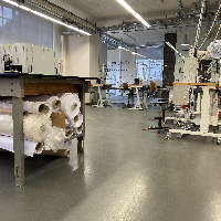
In Figure 1 you see stations consisting of stitching machines, sewing machines, cutters, ovens etc. Processing textile goods nowadays still have a lot hand crafting involved, however to stay competitive, we need a certain amount of automation to lower labor cost. The idea is to use an autonomous guided vehicle to transport pre-processed textile goods from one station to another. This would relieve the workers from leaving their station, so they can concentrate on their textile processing tasks.
We decided that the autonomous guided vehicle will orientate through the learn-factory with a simple camera system. Images from the camera system need to be segmented into parts, such as floor and machine stations. The floor segments of the images are important, so the vehicle knows where to drive, and the machine stations locations are important to find the destination. Segmenting images is a well known problem in machine learning (semantic segmentation) and can be addressed by using neural networks.
Preparation
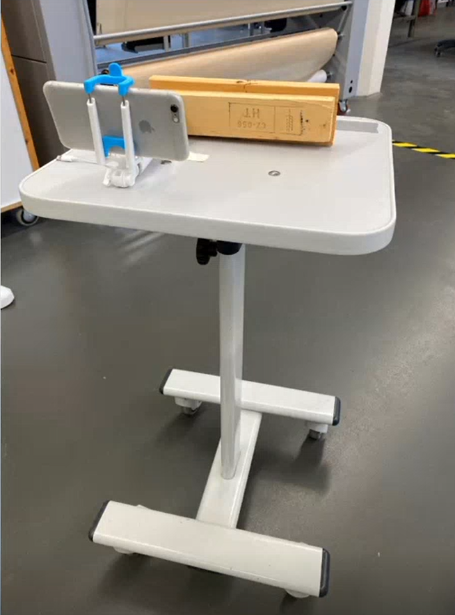
In order to use a neural network to solve the segmentation problem, we need training data. Fortunately this time we have many students helping to create data. The first step is to create images from a perspective of an autonomous guided vehicle. The students mounted a smart phone on a trolley and took images while moving around the trolley, see Figure 2.
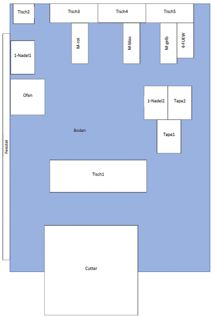
In Figure 3 you see the layout of the learn-factory created by the students. You see the floor in blue, and the stations with their names as white rectangle. The learn-factory was divided into parts from where the images have to be taken. Each part was assigned to one student.
We set the goal, that each student has to take 1000 images from different angles. With 13 participating students, we gathered 13000 images, which we assumed to be a good coverage of the complete learn-factory.
Creating Training Data
Figure 3 shows the layout of the learn-factory with 16 machine and working stations. They are categorized as “1-Nagel1”, “Tape1” etc. You find the complete list of categories in the python dictionary classes below. Also the floor (“Boden”) and the window (“Fenster”) have their assigned categories. Altogether there are 20. Numbers are assigned to each machine and working stations. The number 0 is a category which belongs to neither of the categories in the dictionary classes.
classes = {"1-Nadel1" : 1,
          "1-Nadel2" : 2,
          "Tape1" : 3,
          "Tape2" : 4,
          "Boden" : 5,
          "Tisch0" : 6,
          "Tisch1" : 7,
          "Tisch2" : 8,
          "Tisch3" : 9,
          "Tisch4" : 10,
          "Tisch5" : 11,
          "M-blau" : 12,
          "M-Blau" : 12,
          "M-gelb" : 13,
          "M-Gelb" : 13,
          "M-rot" : 14,
           "M-Rot" : 14,
          "4-FÜW" : 15,
          "4-FUEW" : 15,
          "4-FÃœW" : 15,
          "Fenster" : 16,
          "Ofen" : 17,
          "Cutter" : 18,
          "Heizung" : 19,
         }
As mentioned above every student created 1000 images from the learn-factory. The images need to be process further before training the neural network. We need to tell, which parts of the image belong to which category. See the categories in the code above.
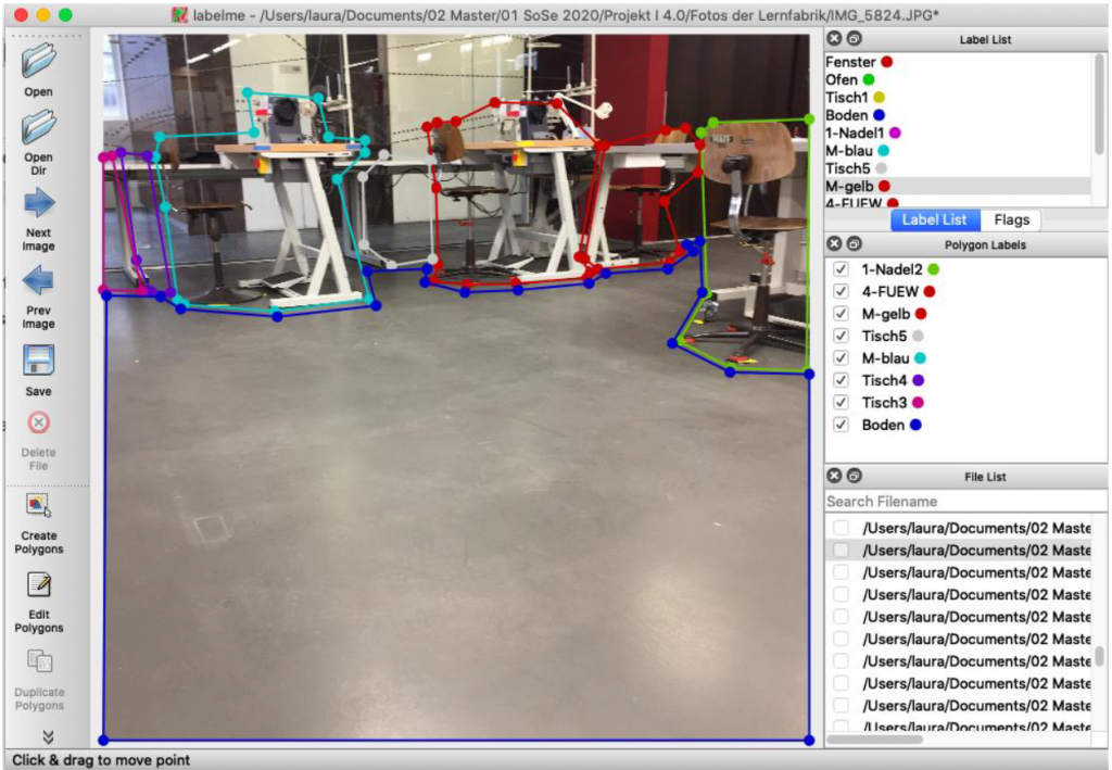
The labelme website offers a downloadable tool to mask parts of the image and assign them to a label (or a category). Figure 4 shows a screenshot of the tool labelme. The student can create closed polygons by marking the vertices with a mouse click. Then the students assign a category to the polygon (Polygon Labels in Figure 4, right side).
The tool labelme saves for each processed image a json file. The json file contains the list of polygons, described by their vertices, the names of the categories, and the image itself, which is saved as a base64 encoded image.
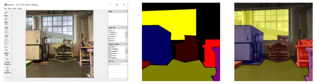
The next step is to process the json files to extract the polygons and their names to create mask images, see Figure 5. On the left side of Figure 5 you see the tool labelme. In the middle you find a processed mask image, created by the polygons. On the right side there is an overlaid image from the original image and the mask image.
Data Processing
Each of the 13 students labeled 1000 images with the tool labelme. The tool labelme generates json files which can be parsed easily with python to extract the vertices of the labeled polygons. Each polygon is assigned to a category (this information can also be extracted from the json file) and each category is assigned a color. The python dictionary color in the code below shows the number/RGB-color assignment.
colors = {0 : (0,0,0),
          1 : (0,0,55),
          2 : (0,0,127),
          3 : (0,55,0),
          4 : (0,127,0),
          5 : (0,127,127),
          6 : (40,0,0),
          7 : (80,0,0),
          8 : (120,0,0),
          9 : (160,0,0),
          10 : (200,0,0),
          11 : (240,0,0),
          12 : (127,0,127),
          13 : (127,127,0),
          14 : (0, 0, 255),
          15 : (0, 255 ,0),
          16 : (0, 255 ,255),
          17 : (100, 0 ,0),
          18 : (200,0,0),
          19 : (255,0,0),
         }

dim = (128, 128)
The function createMasks below is iterating through the list of json-files (13000 files!) located in sourcejsonsdir. In each iteration steps createMasks loads the content of the json file into data. It decodes the image tagged by imageData using the methods b64decode and imdecode and stores it into the variable img. The code verifies if the image is square and resizes it to 128×128.
Next, createMasks is iterating through all polygons in the json file, which are tagged as shapes. Again it iterates through all vertices of each shape and creates a polygon (rr and cc) from them. A mask image is created from the polygon and appended to a list of masks after it is resized to 128×128. The function createMasks sets the values of the pixels which are inside the polygon to the number which corresponds to the category:
mask_orig[rr,cc] = classes[shape[‘label’]]
Finally all masks are added to finalmask by using OpenCV’s threshold and bitwise_and operation. The function createMasks then stores the original image into destimagesdir and the mask image into destmasksdir.
def createMasks(sourcejsonsdir, destimagesdir, destmasksdir):

    assocf = open(os.path.join(path,"assoc_orig.txt"), "w")
    count = 0
    directory = sourcejsonsdir
    for filename in os.listdir(directory):
        if filename.endswith(".json"):
            print("{}:{}".format(count,os.path.join(directory, filename)))

            f = open(os.path.join(directory, filename))
            data = json.load(f)
            img_arr = data['imageData']
            imgdata = base64.b64decode(img_arr)

            img = cv2.imdecode(np.frombuffer(imgdata, dtype=np.uint8), flags=cv2.IMREAD_COLOR)

            assert (img.shape[0] > dim[0])
            assert (img.shape[1] > dim[0])

            if img.shape[0] != img.shape[1]:
                print("shape is wrong: {},{} ... skipping".format(img.shape[0],img.shape[1]))
                continue

            img_resized = cv2.resize(img, dim, interpolation = cv2.INTER_NEAREST)

            finalmask = np.zeros((img_resized.shape[0], img_resized.shape[1]), 'uint8')
            mthresh = np.zeros((img_resized.shape[0], img_resized.shape[1]), 'uint8')
            masks=[]

            for shape in data['shapes']:
                assert(shape['label'] in classes)

                vertices = np.array([[point[1],point[0]] for point in shape['points']])
                vertices = vertices.astype(int)

                rr, cc = polygon(vertices[:,0], vertices[:,1], img.shape)
                mask_orig = np.zeros((img.shape[0], img.shape[1]), 'uint8')
                mask_orig[rr,cc] = classes[shape['label']]
                masks.append(cv2.resize(mask_orig, dim, interpolation = cv2.INTER_NEAREST))

            for m in masks:
                _,mthresh = cv2.threshold(m,1,255,cv2.THRESH_BINARY_INV)
                finalmask = cv2.bitwise_and(finalmask,finalmask,mask = mthresh)
                finalmask += m

            cv2.imwrite(os.path.join(destimagesdir, "{:05d}o.png".format(count)), img_resized)
            cv2.imwrite(os.path.join(destmasksdir, "{:05d}o.png".format(count)), finalmask)

            assocf.write("{:05d}o:{}\n".format(count, data['imagePath']))
            assocf.flush()
            count += 1

        else:
            continue
    f.close()
13000 mask images can now be used for training, just by processing the available data. However, we decided to generate more training data by using data augmentation. The function createMasksAugmented below works in a similar way as createMasks, therefore we just explain a few differences. The function createMasksAugmented rotates the original image with a random angle between -3 and 3 degrees and zooms into the rotated images with a random percentage (between 80 and 90 percent of the original image). The method imutils.rotate_bound is performing this operation. The final image is stored into image_zoomed. The mask image is generated the same way as in function createMasks. However createMasksAugmented rotates and zooms the mask image in the same way as the original image. More data augmentation is applied by OpenCV’s convertScaleAbs method. It modifies randomly contrast and brightness on the rotated and zoomed image before saving it into the destimagedir directory. The rotated and zoomed mask image is saved into the directory destmaskdir.
def createMasksAugmented(sourcejsonsdir, destimagesdir, destmasksdir):

    assocf = open(os.path.join(path,"assoc_augmented.txt"), "w")

    count = 0
    directory = sourcejsonsdir
    for filename in os.listdir(directory):
        if filename.endswith(".json"):
            print("{}:{}".format(count,os.path.join(directory, filename)))

            f = open(os.path.join(directory, filename))
            data = json.load(f)
            img_arr = data['imageData']
            imgdata = base64.b64decode(img_arr)

            img = cv2.imdecode(np.frombuffer(imgdata, dtype=np.uint8), flags=cv2.IMREAD_COLOR)

            assert (img.shape[0] > dim[0])
            assert (img.shape[1] > dim[0])

            if img.shape[0] != img.shape[1]:
                print("shape is wrong: {},{} ... skipping".format(img.shape[0],img.shape[1]))
                continue

            zoom = randint(80,90)/100.0
            angle = (2*random()-1)*3.0
            img_rotated = imutils.rotate_bound(img, angle)

            xf = int(img_rotated.shape[0]*zoom)
            yf = int(img_rotated.shape[1]*zoom)

            img_zoomed = np.zeros((xf, yf, img_rotated.shape[2]), 'uint8')
            img_zoomed[:,:,:] = img_rotated[int((img_rotated.shape[0]-xf)/2):int((img_rotated.shape[0]-xf)/2)+xf,int((img_rotated.shape[1]-yf)/2):int((img_rotated.shape[1]-yf)/2)+yf,:]


            img_resized = cv2.resize(img_zoomed, dim, interpolation = cv2.INTER_NEAREST)

            finalmask = np.zeros((img_resized.shape[0], img_resized.shape[1]), 'uint8')
            mthresh = np.zeros((img_resized.shape[0], img_resized.shape[1]), 'uint8')
            masks=[]

            for shape in data['shapes']:
                assert(shape['label'] in classes)

                vertices = np.array([[point[1],point[0]] for point in shape['points']])
                vertices = vertices.astype(int)

                rr, cc = polygon(vertices[:,0], vertices[:,1], img.shape)
                mask_orig = np.zeros((img.shape[0], img.shape[1]), 'uint8')
                mask_orig[rr,cc] = classes[shape['label']]

                mask_rotated = imutils.rotate_bound(mask_orig, angle)

                mask_zoomed = np.zeros((xf, yf), 'uint8')
                mask_zoomed[:,:] = mask_rotated[int((img_rotated.shape[0]-xf)/2):int((img_rotated.shape[0]-xf)/2)+xf,int((img_rotated.shape[1]-yf)/2):int((img_rotated.shape[1]-yf)/2)+yf]

                masks.append(cv2.resize(mask_zoomed, dim, interpolation = cv2.INTER_NEAREST))

            for m in masks:
                _,mthresh = cv2.threshold(m,1,255,cv2.THRESH_BINARY_INV)
                finalmask = cv2.bitwise_and(finalmask,finalmask,mask = mthresh)
                finalmask += m

            alpha = 0.8 + 0.4*random();
            beta = int(random()*15)

            img_adjusted = cv2.convertScaleAbs(img_resized, alpha=alpha, beta=beta)

            cv2.imwrite(os.path.join(destimagesdir, "{:05d}a.png".format(count)), img_adjusted)
            cv2.imwrite(os.path.join(destmasksdir, "{:05d}a.png".format(count)), finalmask)

            assocf.write("{:05d}a:{}\n".format(count, data['imagePath']))
            assocf.flush()
            count += 1

        else:
            continue
    f.close()
The function createMasksAugmented was applied one time to all available data. So at the end we had 26000 images for training. Since createMasksAugmented uses random numbers for rotation, zooming, brightness and contrast, it could be applied even more than one time.
The UNET Model
We train our data on a UNET model, because we had good semantic segmentation results with this kind of model in previous projects. Hence, the neural network was already described in previous posts. Originally we took the code from here, however modified it slightly to match our purpose. The first function is conv2d_block which executes two convolutions and relu-activation operations in a row, see code below.
def conv2d_block(input_tensor, n_filters, kernel_size=3, batchnorm=True):
    # first layer
    x = Conv2D(filters=n_filters, kernel_size=(kernel_size, kernel_size), kernel_initializer="he_normal",
               padding="same")(input_tensor)
    if batchnorm:
        x = BatchNormalization()(x)
    x = Activation("relu")(x)
    # second layer
    x = Conv2D(filters=n_filters, kernel_size=(kernel_size, kernel_size), kernel_initializer="he_normal",
               padding="same")(x)
    if batchnorm:
        x = BatchNormalization()(x)
    x = Activation("relu")(x)
    return x
The code get_unet below builds up the model by calling conv2_block and maxpooling2D several times (this is called the contracting path). The output of maxpooling2D operations are stored in variables (c1, c2, c3, c4) which are fed later into the expansive path. At the expansive path, get_unet calls reverse convolution operations and concatenates the saved variables (c1, c2, c3, c4) from the contracting path with the output of the Conv2DTranspose operations. In the line:
c10 = Conv2D(len(colors), (1, 1), activation=”softmax”) (c9)
you find the minor change we made. The output size of the model will be an image of size 128×128 with 20 (which is len(color)) layers.
def get_unet(input_img, n_filters=16, dropout=0.5, batchnorm=True):
    # contracting path
    c1 = conv2d_block(input_img, n_filters=n_filters*1, kernel_size=3, batchnorm=batchnorm)
    p1 = MaxPooling2D((2, 2)) (c1)
    p1 = Dropout(dropout*0.5)(p1)

    c2 = conv2d_block(p1, n_filters=n_filters*2, kernel_size=3, batchnorm=batchnorm)
    p2 = MaxPooling2D((2, 2)) (c2)
    p2 = Dropout(dropout)(p2)

    c3 = conv2d_block(p2, n_filters=n_filters*4, kernel_size=3, batchnorm=batchnorm)
    p3 = MaxPooling2D((2, 2)) (c3)
    p3 = Dropout(dropout)(p3)

    c4 = conv2d_block(p3, n_filters=n_filters*8, kernel_size=3, batchnorm=batchnorm)
    p4 = MaxPooling2D(pool_size=(2, 2)) (c4)
    p4 = Dropout(dropout)(p4)

    c5 = conv2d_block(p4, n_filters=n_filters*16, kernel_size=3, batchnorm=batchnorm)

    # expansive path
    u6 = Conv2DTranspose(n_filters*8, (3, 3), strides=(2, 2), padding='same') (c5)
    u6 = concatenate([u6, c4])
    u6 = Dropout(dropout)(u6)
    c6 = conv2d_block(u6, n_filters=n_filters*8, kernel_size=3, batchnorm=batchnorm)

    u7 = Conv2DTranspose(n_filters*4, (3, 3), strides=(2, 2), padding='same') (c6)
    u7 = concatenate([u7, c3])
    u7 = Dropout(dropout)(u7)
    c7 = conv2d_block(u7, n_filters=n_filters*4, kernel_size=3, batchnorm=batchnorm)

    u8 = Conv2DTranspose(n_filters*2, (3, 3), strides=(2, 2), padding='same') (c7)
    u8 = concatenate([u8, c2])
    u8 = Dropout(dropout)(u8)
    c8 = conv2d_block(u8, n_filters=n_filters*2, kernel_size=3, batchnorm=batchnorm)

    u9 = Conv2DTranspose(n_filters*1, (3, 3), strides=(2, 2), padding='same') (c8)
    u9 = concatenate([u9, c1], axis=3)
    u9 = Dropout(dropout)(u9)
    c9 = conv2d_block(u9, n_filters=n_filters*1, kernel_size=3, batchnorm=batchnorm)

    c10 = Conv2D(len(colors), (1, 1), activation="softmax") (c9)

    model = Model(inputs=[input_img], outputs=[c10])
    return model
We mentioned above that we created mask images from the json files, which have a size of 128×128. Each category is simply assigned a number between 0 and 19 at each pixel position. However the neural network has an output of 128x128x20. We use for the neural network a different mask representation, because this way it is preferred for training. Hence, each layer of the 128x128x20 image gets its own category assigned. If a pixel of an image layer is one, it marks the position of an object with its category; if the pixel is zero, it marks that no object of the former category is at this position. Since this is a preferred representation for neural networks, we need to convert the 128×128 masks (created from json files) to 128x128x20 masks. The function makecolormask below is performing this operation. Note that there are more efficient ways to convert the masks, but this will be discussed in a later post.
def makecolormask(mask):
    ret_mask = np.zeros((mask.shape[0], mask.shape[1], len(colors)), 'uint8')
    for i in range(mask.shape[0]):
        for j in range(mask.shape[1]):
                assert(mask[i,j] < len(colors))
                ret_mask[i,j,mask[i,j]] = 1
    return ret_mask
In this project we ran into a problem, which we have not seen in previous projects yet. As mentioned above, we generated 26000 original images and 26000 mask images. Loading all images into memory and with a 8GB NVIDIA graphic card will break the training. Therefore we created the function generatebatchdata to load original and mask images in smaller batches into memory, see code below. The parameters of the functions are fullpathimages and fullpatchmasks which point to the directories of the training data. The lists imagenames and masknames contain the filenames of the original and mask images.
The function generatebatchdata reads the data in (cv2.imread) and appends the data to imagelist and masklist. Here the makecolormask function is applied to convert the json mask image to a 128x128x20 representation. The original images are processed even further with a mean and a standard deviation operations for normalization. Finally the imagelist and masklist is returned with the yield function. Obviously generatebatchdata is executed concurrently. The yield function stops the execution, until the training process continues to execute generatebatchdata with the next batch.
def generatebatchdata(batchsize, fullpathimages, fullpathmasks, imagenames, masknames):

    assert(len(imagenames) == len(masknames))

    while True:
        batchstart = 0
        batchend = batchsize

        while batchstart < len(imagenames):

            imagelist = []
            masklist = []

            limit = min(batchend, len(imagenames))

            for i in range(batchstart, limit):
                if imagenames[i].endswith(".png"):
                    imagelist.append(cv2.imread(os.path.join(fullpathimages,imagenames[i]),cv2.IMREAD_COLOR ))
                if masknames[i].endswith(".png"):
                    masklist.append(makecolormask(cv2.imread(os.path.join(fullpathmasks,masknames[i]),cv2.IMREAD_UNCHANGED )))


            train_data = np.array(imagelist, dtype=np.float32)
            train_mask= np.array(masklist, dtype=np.float32)

            train_data -= train_data.mean()
            train_data /= train_data.std()

            yield (train_data,train_mask)

            batchstart += batchsize
            batchend += batchsize
In the code below you see that the function generatebatchdata is instantiated twice. One time for training data, and one time for validation data. Previously we selected randomly about 15% of the original and mask images and moved them to validation directories (fullpathimagesvalid and fullpathmasksvalid).
generator_train = generatebatchdata(30, fullpathimages, fullpathmasks, imagenames, masknames)
generator_valid = generatebatchdata(30, fullpathimagesvalid, fullpathmasksvalid,  imagenamesvalid, masknamesvalid)
The UNET model is instantiated and compiled in the code below. As input the model expects images with dimension dim with three layers (RGB) which is 128x128x3.
input_img = Input((dim[0], dim[1], 3), name='img')
model = get_unet(input_img, n_filters=len(colors), dropout=0.05, batchnorm=True)
model.compile(optimizer=Adam(), loss="categorical_crossentropy", metrics=["accuracy"])
During training we use three callback function. The first callback is EarlyStopping, which stops the training process if there is no improvement of the loss value after ten epochs. The next callback ReduceLROnPlateau modifies the learning rate if there is no imrovement concerning loss after three epochs. The last callback ModelCheckpoint saves a checkpoint of the model during the training process if the model has improved its loss value.
callbacks = [
    EarlyStopping(patience=10, verbose=1),
    ReduceLROnPlateau(factor=0.1, patience=3, min_lr=0.00001, verbose=1),
    ModelCheckpoint(os.path.join(path, dirmodels,"model-chkpt.h5"), verbose=1, save_best_only=True, save_weights_only=True)
]
Below the code starts the training process. The training was executed on a NVIDIA 2070 graphic card with 8GB memory. It turned out that we have a accuracy of 95,3% and a validation accuracy of 94,9%. So we have a small overfitting. Training time was about 20 minutes.
model.fit_generator(generator_train,steps_per_epoch=530, epochs=20, callbacks=callbacks, validation_data=generator_valid, validation_steps=3064)
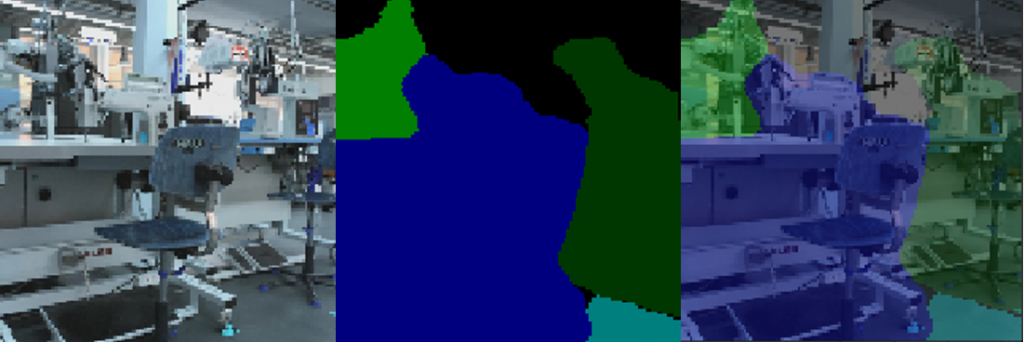
The function predictedmask below is a utility function to create mask images from the model’s output back to the original mask image form we received after processing the json files. It is a reverse function of makecolormask. The function predictedmask is useful to create masks as seen as in Figure 6 (in the middle) for display purpose. Since 128x128x20 images cannot be displayed in such a way.
def predictedmask(masklist):
    y_list = []
    for mask in masklist:
        assert mask.shape == (dim[0], dim[1], 20)
        imgret = np.zeros((dim[0], dim[1]), np.uint8)
        for i in range(dim[0]):
            for j in range(dim[1]):
                result = np.where(mask[i,j,:] == np.amax(mask[i,j,:]))
                assert result[0][0] < len(colors)
                imgret[i,j] = result[0][0]
        y_list.append(imgret)
    return y_list
Figure 6 shows a verification example. An original image (left) was put into the trained model with the model’s predict method (model.predict) and the result can be seen in Figure 6 in the middle. The function predictedmask was applied here. Overlaying the left and the middle image results to the right image.
Creating an augmented video
The goal of this project is to create an augmented life video from the learn-factory while walking through with a video camera. The application should mask the floor, and the machines should be labeled with text, which are the categories. Basically each image of the video is fed into the trained neural network and it predicts a 128x128x20 mask image. However, further processing is needed, such as labeling the video images with text.
The function predictedmask above converts 128x128x20 mask images back to 128×128 mask images. The pixel values are values between 0 and 19. The python dictionary categories below shows an assignment between the values and the categories written as text. A similar assignment (python dictionary classes) we have above, but here it is just the way around.
categories = {1: "1-Nadel1",
              2: "1-Nadel2",
              3: "Tape1",
              4: "Tape2",
              5: "Boden",
              6: "Tisch0",
              7: "Tisch1",
              8: "Tisch2",
              9: "Tisch3",
              10: "Tisch4",
              11: "Tisch5",
              12: "M-Blau",
              13: "M-Gelb",
              14: "M-Rot",
              15: "4-FUW",
              17: "Ofen",
              18: "Cutter",
              19: "Heizung",
         }
As already mentioned, the masks created by predictedmask are one layer images, whose pixels values are between 0 and 19. In order to convert the masks to a color image the function makemaskcolor is used. It uses the python dictionary colors to assign each pixel value to a color value. The output of makemaskcolor is a colored mask image of one category with shape 128x128x3. The parameter color indicates from which category a mask should be created. Such as, if you want the mask of a floor (Boden, see python dictionary categories), the value of color should be five. In a later post, we can show how this operation can be done more efficient.
def makemaskcolor(mask, color):
    ret_mask = np.zeros((mask.shape[0], mask.shape[1], 3), 'uint8')
    for i in range(mask.shape[0]):
        for j in range(mask.shape[1]):
                if mask[i,j] == color:
                    ret_mask[i,j,0] = colors[color][0]
                    ret_mask[i,j,1] = colors[color][1]
                    ret_mask[i,j,2] = colors[color][2]
    return ret_mask
Below the code of the function markpicture. The input parameter inp_img is a mask image from the predictedmask ouput. The parameter orig_img is the original image, which has been fed into the neural network model for the mask prediction. We decided to show only the mask of the floor. The function markpicture creates with the following code the floor mask (boden stands for floor):
boden = makemaskcolor(inp_img,5)
Then the function markpicture iterates through the category values, however it omits 5 and 16. The category 16 is a window (Fenster stands for window) and needs no label. OpenCV’s inRange Method extracts the i’th mask (see for loop) and assigns it to inp_img_new. The code calls OpenCV’s findContour to get the contour of the i’th category. The contour needs to exceed a minimum area, which can be determined by cv2.contourArea. The code then calculates the center of gravity of the contour and puts text indicating the category at this position onto the original image. Text is put two times there; first white text with a larger boldness and second text in color of the category (see dictionary color) and a smaller boldness. By doing this, we improve to emphasize the text on the image. Finally markpicture overlays the processed image with the floor (cv2.addWeighted) and returns the image.
def markpicture(inp_img, orig_img):

    update_img = orig_img.copy()

    img_new = np.zeros((inp_img.shape[0], inp_img.shape[1],3), 'uint8')
    inp_img_new = np.zeros((inp_img.shape[0], inp_img.shape[1],3), 'uint8')
    boden = np.zeros((inp_img.shape[0], inp_img.shape[1],3), 'uint8')
    boden_resized = np.zeros((orig_img.shape[0], orig_img.shape[1],3), 'uint8')
    weighted = np.zeros((orig_img.shape[0], orig_img.shape[1],3), 'uint8')

    boden = makemaskcolor(inp_img,5)

    for i in [1,2,3,4,6,7,8,9,10,11,12,13,14,15,17,18,19]:

        inp_img_new = inp_img.copy()
        inp_img_new = inp_img_new.astype(np.uint8)

        inp_img_new = cv2.inRange(inp_img_new,i,i)
        contours,_ = cv2.findContours(inp_img_new,cv2.RETR_TREE,cv2.CHAIN_APPROX_NONE)

        if len(contours) > 0:

            contours = sorted(contours, key=cv2.contourArea,  reverse=True)

            M = cv2.moments(contours[0])
            area = cv2.contourArea(contours[0])
            if M['m00'] > 0 and area > 600:

                cx = int(int(M['m10']/M['m00'])*orig_img.shape[0]/inp_img.shape[0])
                cy = int(int(M['m01']/M['m00'])*orig_img.shape[1]/inp_img.shape[1])
                update_img= cv2.putText(update_img,categories[i],(cx,cy), cv2.FONT_HERSHEY_SIMPLEX,0.5 if area > 800 else 0.25, (255,255,255), 4)
                update_img= cv2.putText(update_img,categories[i],(cx,cy), cv2.FONT_HERSHEY_SIMPLEX,0.5 if area > 800 else 0.25, colors[i], 2 if area > 500 else 1)

    boden_resized = cv2.resize(boden, (orig_img.shape[0], orig_img.shape[1]), interpolation = cv2.INTER_AREA)

    assert(boden_resized.shape == update_img.shape)
    cv2.addWeighted(update_img, 0.6, boden_resized, 0.4, 0, weighted)

    return weighted
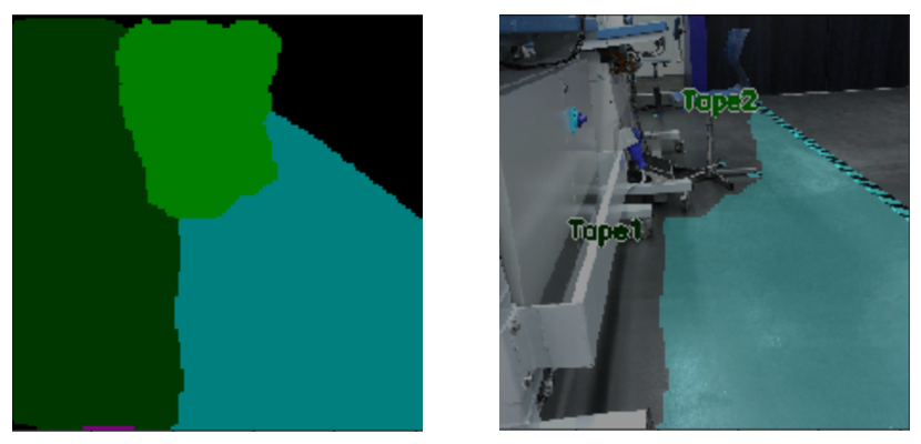
In Figure 7 you can find an output of maskpicture. On the left side a representation of the mask from the neural network prediction and on the right side a processed original image with text and overlaid floor. You find here the text of the categories Tape1 and Tape2.
To create an augmented video we used the code below. Before augmentation we walked through the learn-factory and created a normal video from a robot’s perspective and named it video.mp4. OpenCV’s VideoCapture opens the video and iterates through it image by image. VideoCaputure’s read method extracts each image from the video and assigns it to frame. frame is resized and normalized. Then the code feeds it into the neural network’s predict method. The output is a predicted mask (with shape 128x128x20), which is converted to another mask representation with the function predictedmask (shape 128×128). Its output is fed into markpicture, which is putting text on the image and marking the floor. Finally the image is written to a new video videounet128-1.mp4.
cap = cv2.VideoCapture(os.path.join(path,"videos",'video.mp4'))
if (cap.isOpened() == True):

    print("Opening video stream or file")
    out = cv2.VideoWriter(os.path.join(path,"videos",'videounet128-1.mp4'),cv2.VideoWriter_fourcc(*'MP4V'), 25, (256,256))
    while(cap.isOpened()):
        ret, frame = cap.read()

        if ret == False:
            break

        frame_resized = np.zeros((dim[0], dim[1], 3), 'uint8')
        frame_resized = cv2.resize(frame, (dim[0],dim[1]), interpolation = cv2.INTER_AREA)
        test_data = []
        test_data.append(frame_resized)
        test_data = np.array(test_data, dtype=np.float32)
        test_data -= test_data.mean()
        test_data /= test_data.std()

        predicted = model.predict(test_data, batch_size=1, verbose=0)
        assert(len(predicted) == 1)
        pmask = predictedmask(predicted[0])

        if ret == True:
            img = markpicture(pmask, frame)
            out.write(img)
            cv2.imshow('Frame',img)
            if cv2.waitKey(25) & 0xFF == ord('q'):
                break

    out.release()

cap.release()
cv2.destroyAllWindows()
Conclusion
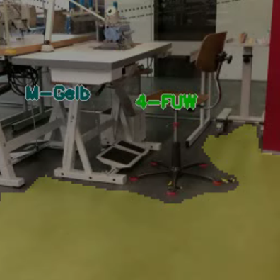
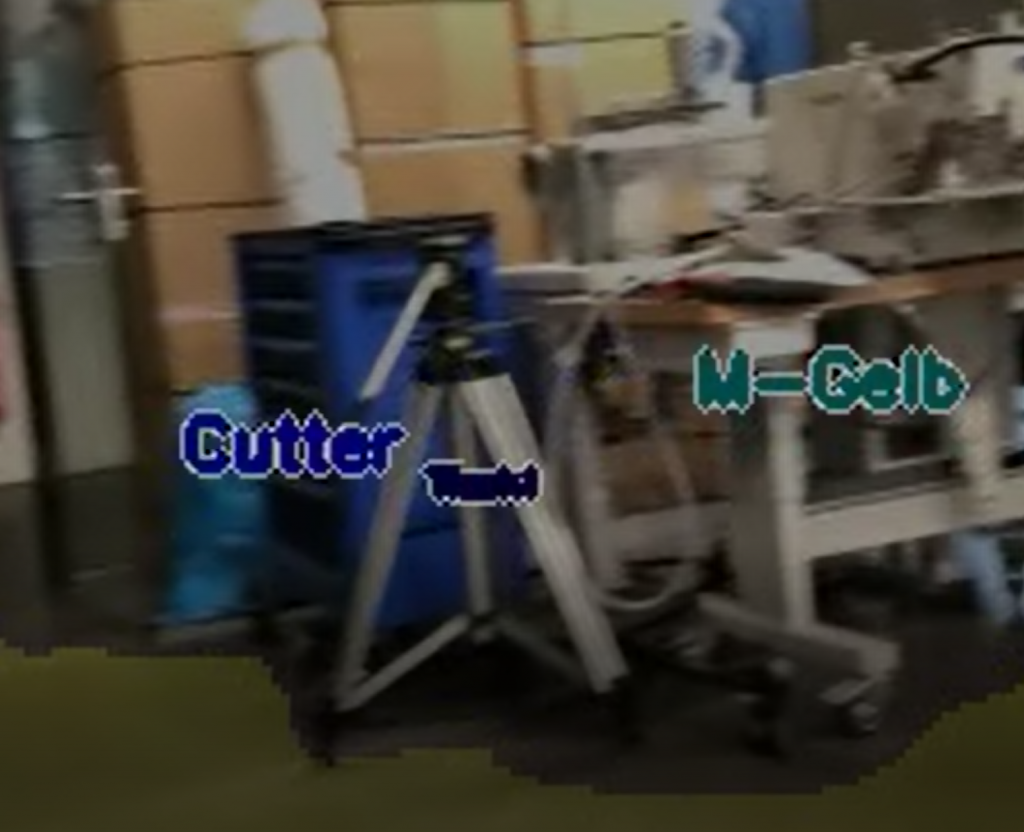
The resulting videos are astonishing. You can walk through the learn-factory with a video camera and process in real-time the video and you receive an output such as displayed in Figure 8. The machines are mostly labeled correctly and the floor indicates where a autonomous guided vehicle could drive.
There are situations where the labeling works not correctly, especially if you walk into areas, where the students have not taken any pictures and therefore no labeling was done. In Figure 3 it is the area on the right side. Figure 9 shows such a snapshot where the labeling is completely incorrect. However the floor is still predicted correctly. Note that no training data existed for this area, so the chaotic prediction is expected.
Acknowledgement
Special thanks to the class of Summer Semester 2020 Forschungsprojekt Industrie 4.0 providing the images of the learn-factory (13000!) and labeling the images for the training data (also 13000!!) used for the neural network. We appreciate this very much, and we know how much effort you have put into this.
Also special thanks to the University of Applied Science Albstadt-Sigmaringen for hosting the learn-factory and providing the appliances to enable this research.