Introduction
Once a year we offer a class called Forschungsprojekt Industrie 4.0 (Research Project 4.0), which is a practical assignment to enrolled of students. This time the goal of the assignment was to create a quality control system which recognizes errors and breaks on textile seams. Six students enrolled to this specific assignment.
In Figure 1 you see on the left upper side a sewing machine from top. We reconstructed a lamp holder to a camera holder by attaching a usb-camera (1 on Figure 1) on it. Then we moved the usb-camera right next to the sewing machine (2 on Figure 1) to have a camera view of the sewed textile.
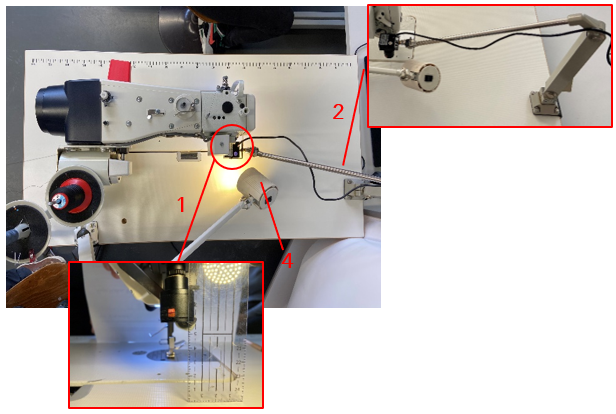
While the sewing maching is running, the usb-camera takes images from the textile with its sewed string. The image is sent to a quality control system, which should recognize errors and breaks. So the assignment for the students here is to create a quality control system.
Preparations
We decided to use a neural network to recognize breaks and errors from the images made by the usb-camera. For training the neural network the students needed to gather numerous training images.
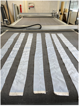
For this purpose the students cut textile stripes which can bee seen in Figure 2. Then the students sewed seams along the textile stripes, which were recorded by the usb-camera system at the same time. The videos were saved as mp4 files.
Only in rare cases sewing machines produce errors or breaks. This is why we had to generate the errors and breaks ourselves.
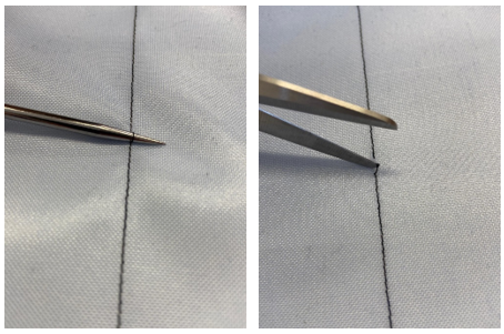
In Figure 3 you can see how we create errors and breaks. The left picture shows how an error is produced by sticking a scissor under the seam which widening the string. The right picture shows how we produce a break by cutting the string with the scissor. Therefore we have already two categories to distinguish: “errors” and “breaks”. We call them from now on attributes. There are two more attributes to come.
On sewing machines you can set up the distances for the stitches. Possible values are e.g. 2mm or 4mm. We decided to use exactly these values to distinguish and defined for this the attribute “length”. If the attribute “length” is true, than we have a stitch distance of 2mm, if false we have a stitch distance of 4mm.
The last attribute we call “good”. This simply means that we recognize the image on the seam as a good seam. If attribute “good” is set to false, there is a problem with an “error”, “break” or “length”. This makes it altogether four attributes: “good”, “error”, “break” and “length”.
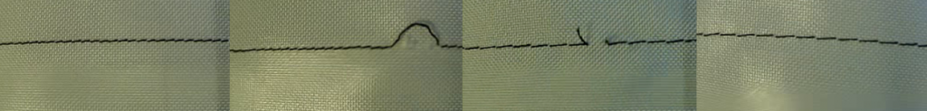
In Figure 4 you find images for each attribute. On the left you find a “good” image. The second left picture you see an “error”. On the second right picture you find a “break”. The right most picture shows a length distance of 4mm, which is an attribute with value false.
You might have noticed that the picture on the right and the picture on the second right have the same stitch distance. So the second left picture has a “break”, and a stitch distance of 4mm. This means the classifications are not exclusive. An image from the usb-camera can show all attributes as true, all attributes as false or any other combination.
Creating labeled data
In Figure 1 you can see the setup of the sewing machine and the attached usb-camera. We used this setup to create videos while sewing strings on the textile stripes (Figure 2). Since error’s and break’s do not happen very often, we prepared the textile stripes with the scissor, and created new videos from them. Our goal was to have balanced data, which means that there is a good proportion of error’s and break’s in our data set. We are not describing the code to create video’s here. You could actually use any cell phone for this task.
However we want to show how we have labeled the training images resulting from the videos. The code below sets the basepath and assigns the video file path to the variable video. We will also use a file called data.csv to store the values (true or false) for each attribute on every image. It is basically a lookup table. The filename is assigned to datacsv.
basepath = r"..."
videos = "videos"
videopath = os.path.join(basepath,videos)

videonamepre = "video_2021_05_05_09_34_57__2mm_Kombi"
videonameext = "mp4"
datacsv = videonamepre + "_data.csv"
videoname = videonamepre + "." + videonameext
video = os.path.join(videopath,videoname)
The list picnames contains the names of the attributes, see code below. The list picstats contain the true or false values of the attributes for one image. The variable picpath is the path of the directory where we store our images extracted from the videos.
picnames = ["good","error","break","length"]
picstats = [False, False, False, False]

picspath = os.path.join(basepath, "pics")
The function save_entry is shown below. It uses the python library pandas to append the classification information (parameters name, picnames and picstats) to a data.csv file. First it creates a data frame, then it reads in an already existing data.csv file and loads in its content into the list datalist. Finally it moves the name, picnames and picstats values into the dictionary dataitem and appends it to datalist. The function save_entry converts datalist into a pandas data frame and saves the content into the data.csv file.
def save_entry(name, picnames, picstats):

    arr = os.listdir(picspath)

    df = pd.DataFrame()
    datalist = []


    if os.path.isfile(os.path.join(os.path.join(picspath,datacsv))):

        df=pd.read_csv(os.path.join(os.path.join(picspath,datacsv)))
        for index, row in df.iterrows():
            datalist.append({'name': row['name'], picnames[0]: row[picnames[0]], picnames[1]: row[picnames[1]], picnames[2]: row[picnames[2]], picnames[3]: row[picnames[3]]})

    dataitem ={'name': name, picnames[0]: picstats[0], picnames[1]: picstats[1], picnames[2]: picstats[2], picnames[3]: picstats[3]}
    datalist.append(dataitem)
    df = pd.DataFrame(datalist)
    df.to_csv(os.path.join(picspath, datacsv))

    return
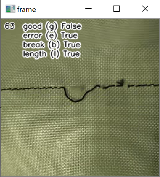
The code below is a small application to label the images from the previously created videos. First it opens a video named video with OpenCV’s constructor VideoCapture. The code runs into a loop to process each single image of the video. The OpenCV’s function waitKey stops the code execution until a key is pressed. In case the user presses the key “n”, the code reads in the next image of the video. It then puts text with classification information onto the image and displays it. Basically it displays the keys g for “good”, e for “error”, b for “break”, l for “length” and their attribute values. The user can press the keys g, e, b, l to toggle the attribute values. If the user presses the s key, then the application saves the attribute values with the function save_entry into the data.csv file.
count = 0
cap = cv2.VideoCapture(video)

if cap.isOpened():
    ret, frame = cap.read()

while(cap.isOpened()):

    if ret == True:
        framedis = frame.copy()
        framedis = cv2.putText(framedis, str(count), (5, 15), cv2.FONT_HERSHEY_SIMPLEX, 0.4, (255,255,255), 2, cv2.LINE_AA)
        framedis = cv2.putText(framedis, str(count), (5, 15), cv2.FONT_HERSHEY_SIMPLEX, 0.4, (0,0,0), 1, cv2.LINE_AA)
        framedis = cv2.putText(framedis, picnames[0] + " (g) " + str(picstats[0]), (35, 15), cv2.FONT_HERSHEY_SIMPLEX, 0.4, (255,255,255), 3, cv2.LINE_AA)
        framedis = cv2.putText(framedis, picnames[0] + " (g) " + str(picstats[0]), (35, 15), cv2.FONT_HERSHEY_SIMPLEX, 0.4, (0,0,0), 1, cv2.LINE_AA)
        framedis = cv2.putText(framedis, picnames[1] + " (e) " + str(picstats[1]), (35, 30), cv2.FONT_HERSHEY_SIMPLEX, 0.4, (255,255,255), 3, cv2.LINE_AA)
        framedis = cv2.putText(framedis, picnames[1] + " (e) " + str(picstats[1]), (35, 30), cv2.FONT_HERSHEY_SIMPLEX, 0.4, (0,0,0), 1, cv2.LINE_AA)
        framedis = cv2.putText(framedis, picnames[2] + " (b) " + str(picstats[2]), (35, 45), cv2.FONT_HERSHEY_SIMPLEX, 0.4, (255,255,255), 3, cv2.LINE_AA)
        framedis = cv2.putText(framedis, picnames[2] + " (b) " + str(picstats[2]), (35, 45), cv2.FONT_HERSHEY_SIMPLEX, 0.4, (0,0,0), 1, cv2.LINE_AA)
        framedis = cv2.putText(framedis, picnames[3] + " (l) " + str(picstats[3]), (35, 60), cv2.FONT_HERSHEY_SIMPLEX, 0.4, (255,255,255), 3, cv2.LINE_AA)
        framedis = cv2.putText(framedis, picnames[3] + " (l) " + str(picstats[3]), (35, 60), cv2.FONT_HERSHEY_SIMPLEX, 0.4, (0,0,0), 1, cv2.LINE_AA)

        cv2.imshow('frame',framedis)
    else:
        break

    key = cv2.waitKey(0) & 0xFF
    if key == ord('q'):
        break
    if key == ord('n'):
        ret, frame = cap.read()
        count += 1
    if key == ord('g'):
        if picstats[0] == True:
            picstats[0] = False
        else:
            picstats[0] = True
    if key == ord('e'):
        if picstats[1] == True:
            picstats[1] = False
        else:
            picstats[1] = True
    if key == ord('b'):
        if picstats[2] == True:
            picstats[2] = False
        else:
            picstats[2] = True
    if key == ord('l'):
        if picstats[3] == True:
            picstats[3] = False
        else:
            picstats[3] = True


    if key == ord('s'):
        save_entry(videonamepre+f"_{count}.png", picnames, picstats)
        cv2.imwrite(os.path.join(picspath, videonamepre+f"_{count}.png"),frame)

cap.release()
cv2.destroyAllWindows()
In Figure 5 you can see how the application displays the current image of a video. The user can change the attribute values by pressing one of the described keys to save each image into the data.csv file.
The students working on this project created around 15000 images and saved their attribute values with this application into csv files.
Preprocessing the data
For training we need to have both, training data and validation data, which we want to separate. We do this by creating two files with lookup tables, a train.csv file and a valid.csv file. Both files have the image file name, the path location and its attribute values. Also we take a small number of images and assign them to a test data file which we call test.csv.
The function createcsv below is creating a new csv file with a csv file name as parameter (datacsv) from a list piclist. The list piclist contains a list of image filenames and its attribute values.
def createcsv(datacsv, targetpath, piclist):

    datalist = []

    df = pd.DataFrame()

    for item in piclist:
        datalist.append({'name': item[0], classes[0]: item[1][classes[0]], classes[1]: item[1][classes[1]], classes[2]: item[1][classes[2]], classes[3]: item[1][classes[3]]})

    df = pd.DataFrame(datalist)
    df.to_csv(os.path.join(targetpath, datacsv))
The code below opens all csv files one by one located inside the fullpathpic directory . It reads each files content and moves it into a pandas dataframe df. The code iterates through the content and moves each entry into the list picnamelist. So each entry of picnamelist contains a full path and filename of the image and its attribute values.
The list picnamelist is then shuffled with random‘s shuffle function and 20 percent of picnamelist elements are moved into validlist. The code moves another two percent of picnamelist elements into testlist, and finally the code moves the remaining content into trainlist (around 78 percent). The code subsequently calls the function createcsv with validlist, testlist and trainlist as parameters to store lookup tables into valid.csv, test.csv and train.csv.
picnamelist = []
attributelist = []
validlist = []
testlist = []
trainlist = []

for file in os.listdir(fullpathpic ):
    if file.endswith(".csv"):
        f = open(os.path.join(os.path.join(fullpathpic,file)), "r")
        df = pd.read_csv(f, index_col = 0)

        for index, row in df.iterrows():
            picname = row["name"]

            if os.path.isfile(os.path.join(fullpathpic, picname)):
                picnamelist.append([os.path.join(fullpathpic, picname), row])


random.shuffle(picnamelist)

num = 20*len(picnamelist) // 100
validlist = picnamelist[:num]
testlist = picnamelist[num:num+num//10]
trainlist =  picnamelist[num+num//10:]

createcsv("valid.csv", basepath, validlist)
createcsv("test.csv", basepath, testlist)
createcsv("train.csv", basepath, trainlist)
Training
The code below defines the basepath, and the location of the lookup tables for the training, validation and testing data (traincsv, validcsv and testcsv). The code stores the model into the path model_path. The model filename is modelsaved. The list classes contains the attributes, like picnames above (note that the code below and above are different code files).
The pandas read_csv function returns the length of the training data and validation data and assigns them to lentrain and lenvalid.
basepath = r"..."
traincsv = os.path.join(basepath, "train.csv")
validcsv = os.path.join(basepath, 'valid.csv')
testcsv = os.path.join(basepath, 'test.csv')
model_path = os.path.join(basepath, 'models')

classes = ["good","error","break","length"]

now = datetime.datetime.now()

modelsaved = "model.h5"

lentrain = pd.read_csv(traincsv, index_col = 0).shape[0]
lenvalid = pd.read_csv(validcsv, index_col = 0).shape[0]
We have described the function generatebatchdata previously here, so we dont go too much into details. As parameter we use the previously created lookup tables and open them with pandas read_csv function. The code moves the filenames into the list filenames and its attribute values into the list classnumbers. During training the number of elements (batchsize elements) are taken from both lists filenames and classnumbers, then the images are opened with OpenCV’s function imread and returned to the training process. Around 70 percent of the images are augmented by its brightness and contrast with OpenCV’s convertScaleAbs function.
def generatebatchdata(batchsize, datacsv, classes):

    filenames = []
    classnumbers = []

    df = pd.read_csv(datacsv, index_col = 0)

    for index, row in df.iterrows():
        filenames.append(row["name"])
        classnumbers.append([int(row[classes[0]]), int(row[classes[1]]), int(row[classes[2]]), int(row[classes[3]])])

    while True:
        batchstart = 0
        batchend = batchsize

        while batchstart < len(filenames):

            imagelist = []
            classlist = []

            limit = min(batchend, len(filenames))

            for i in range(batchstart, limit):
                img = np.zeros((dim[0], dim[1],3), 'uint8')
                img = cv2.resize(cv2.imread(filenames[i],cv2.IMREAD_COLOR ), dim, interpolation = cv2.INTER_AREA)
                if random.random() > 0.3:
                    alpha = 0.8 + 0.4*random.random()
                    beta = int(random.random()*15)
                    img = cv2.convertScaleAbs(img, alpha=alpha, beta=beta)

                imagelist.append(img)
                classlist.append(classnumbers[i])


            train_data = np.array(imagelist, dtype=np.float32)
            train_data -= train_data.mean()
            train_data /= train_data.std()
            train_class= np.array(classlist, dtype=np.float32)

            yield (train_data,train_class)

            batchstart += batchsize
            batchend += batchsize
We instantiate two functions from generatebatchdata: generator_train and generator_valid. We have set the batchsizes for training to 20, and for validation to one.
batchsizetrain = 20
batchsizevalid = 1

generator_train = generatebatchdata(batchsizetrain, traincsv , classes)
generator_valid = generatebatchdata(batchsizevalid, validcsv, classes)
The functions relu_bn, residual_block, and create_res_net in the code below create a residual neural network (RNN). Dorian Lazar supplied the code on github and it can be found here. We are not going to much into details, but the create_res_net is implementing a RNN from elements as shown as in Figure 6. You see here one residual block element in case the downsample parameter was set to true. The function create_res_net is appending several such blocks into one complete RNN.
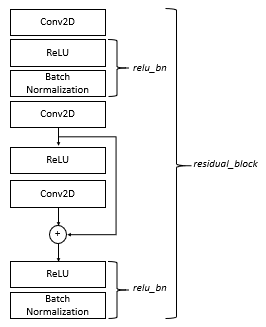
We slightly modified the code at the end of the function create_res_net. As an output we have a dense layer with four neurons, which is the length of the list classes (also of the number of attributes we use). The last activation function we use the sigmoid function. Using the sigmoid function is common practice for mulit-label classfication problems in combination with the binary_crossentropy loss function.
def relu_bn(inputs: Tensor) -> Tensor:
    relu = ReLU()(inputs)
    bn = BatchNormalization()(relu)
    return bn

def residual_block(x: Tensor, downsample: bool, filters: int, kernel_size: int = 3) -> Tensor:
    y = Conv2D(kernel_size=kernel_size,
               strides= (1 if not downsample else 2),
               filters=filters,
               padding="same")(x)
    y = relu_bn(y)
    y = Conv2D(kernel_size=kernel_size,
               strides=1,
               filters=filters,
               padding="same")(y)

    if downsample:
        x = Conv2D(kernel_size=1,
                   strides=2,
                   filters=filters,
                   padding="same")(x)

    out = Add()([x, y])
    out = relu_bn(out)
    return out

def create_res_net():

    inputs = Input(shape=(dim[0], dim[1], 3))
    num_filters = 64

    t = BatchNormalization()(inputs)
    t = Conv2D(kernel_size=3,
               strides=1,
               filters=num_filters,
               padding="same")(t)
    t = relu_bn(t)

    num_blocks_list = [2, 4, 2]
    for i in range(len(num_blocks_list)):
        num_blocks = num_blocks_list[i]
        for j in range(num_blocks):
            t = residual_block(t, downsample=(j==0 and i!=0), filters=num_filters)
        num_filters *= 2

    t = AveragePooling2D(4)(t)
    t = Flatten()(t)
    outputs = Dense(len(classes), activation='sigmoid')(t)

    model = Model(inputs, outputs)

    return model
The code below creates a model with the function create_res_net and assigns it to the variable model. The variable model is compiled with the binary_crossentropy loss function. The summary method shows the structure of the model.
model = create_res_net()
model.compile(Adam(lr=.00001), loss="binary_crossentropy", metrics=['accuracy'])
model.summary()
For training and validation you need to specify the number of steps: steptrainimages and stepsvalidimages. We can calculate them by dividing the number of training images with the batchsize for training and the number of validation images with the batchsize for validation.
stepstrainimages = lentrain//batchsizetrain
stepsvalidimages = lenvalid//batchsizevalid
Below, the code trains the model with its fit method. Parameters are the generators generator_train and generator_valid. Also the number of steps (stepstrainimages and stepsvalidimages) need to be given. After execution, the fit function returns its history content into variables. They can be used to create a checkpoint modelsaved with details on loss, valid_loss, accuracy and val_accuracy. By looking at the model’s checkpoint name, we can see an indication of of quality of the training. The code saves the checkpoint with its save_weights method.
hist = model.fit(generator_train,steps_per_epoch=stepstrainimages, epochs=10, validation_data=generator_valid, validation_steps=stepsvalidimages)

tl=hist.history['loss'][-1]
vl=hist.history['val_loss'][-1]
ta=hist.history['accuracy'][-1]
va=hist.history['val_accuracy'][-1]

modelsaved = f"model_{net}_{tl:.2f}_{vl:.2f}_{ta:1.3f}_{va:1.3f}.h5"
model.save_weights(os.path.join(model_path,modelsaved))
After training we compared the training losses with the validation losses. We find, that the training losses are smaller compared to the validation losses which indicates an overfitting. In the result section below we show the prediction results with testing data.
Result
We created not only a lookup table for training data and validation data, but also for testing data in the file test.csv. We set aside for this around 300 images. Then we ran the 300 images through the prediction method of model and compared the results with the attribute values in the lookup table. We are not showing here the code. Below you find the percentages of correct answers for the attributes “good”, “error”, “break” and “length”. We see that the “length” exceeds 100 percent correctness (all images were predicted concerning attribute “length” correctly). While “error” and “break” have a prediction accuracy of around 97 percent. Only the “good” category has less accuracy. We explain this, because student’s decision for “good” during labeling could be very error prone. Six students can label the attribute “good” very subjectively. While the decision to label an attribute “error”, “break” and “length” is much clearer to make.
Good Accuracy: 82.70270270270271
Error Accuracy: 97.2972972972973
Break Accuracy: 97.02702702702702
Length Accuracy: 100.
To do further validation on the test images, we created heatmaps. A heatmap can point out the pixels, which leads to the neural network’s classification decision. We have described the code for creating heatmaps here, so we will not show it in this post anymore.
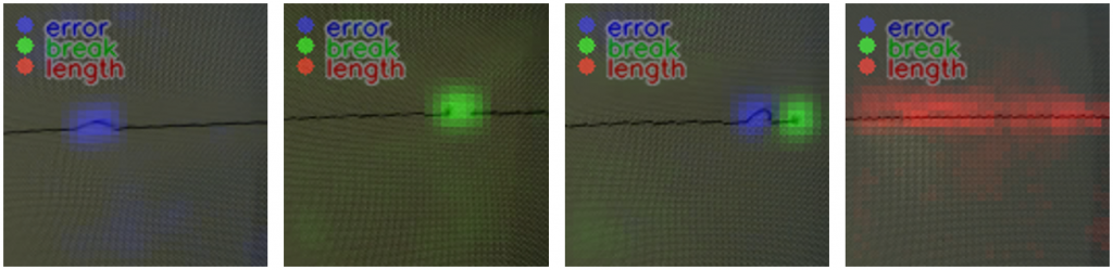
Figure 7 shows four heatsmaps. The left most picture shows correctly an error in blue. This means that the model predicts correctly the pixels around the seam error which led to the right classification decision. The same is true for the second left picture. We have here a break, and the heatmap showing correctly the pixels of the break in green. Since we have multi-label classification, there are cases where we have an error and a break at the same time. The second right picture is showing this case. Also here the decision was made correctly with pixels around the breaks in green and around the error in blue. The most right picture shows the pixels in red, leading to the length decision.
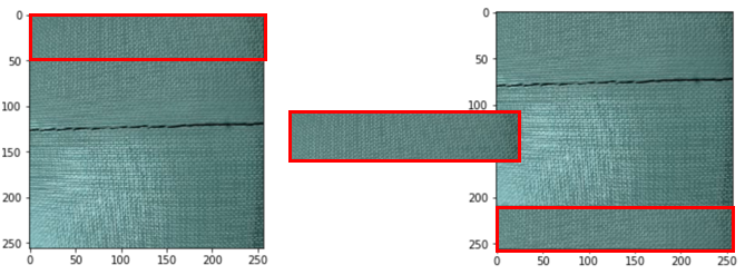
One last remark. The generatebatchdata function we described above did some data augmentation by changing the brightness and the contrast of 70 percent of all images. Actually we did even more data augmentation, which was not shown here. The 15000 images were doubled to 30000 images by modifying them in the following way. We took a portion of the upper image out and appended this portion to the bottom part of the image. You find in Figure 8 an illustration how we did this. These are simple OpenCV functions, so we leave out the code here.
Acknowledgement
Special thanks to the class of Summer Semester 2021 Forschungsprojekt Industrie 4.0 providing 15000 images for the training data used for the neural network training. We appreciate this very much, and we know how much effort you have put into this.
Also special thanks to the University of Applied Science Albstadt-Sigmaringen for hosting the learn-factory and providing the appliances to enable this research.