Chromosomes have one short arm and one long arm. The centromere sits in between and links both arms together. Biologists find it convenient that an application can spot automatically the position of the centromere on a chromosome image. In general for image processing, it is useful for an application to know the centromere position to simplify the classification of the chromosome type.
With this project we want to show how an application can get the centromere positions by using a neuronal network. In order to train the neuronal network, we need sufficient training data. We show here, how we created the training data. A position in an image is a coordinate with two numbers. The application must therefore use an neuronal network with an regression layer as an output. In this post we show what kind of neuronal network we used for retrieving a position from an image.
Creating the Training Data
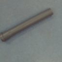
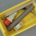
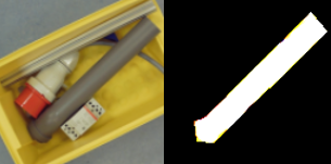
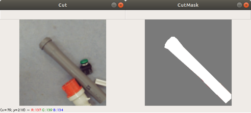
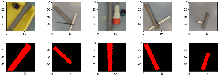
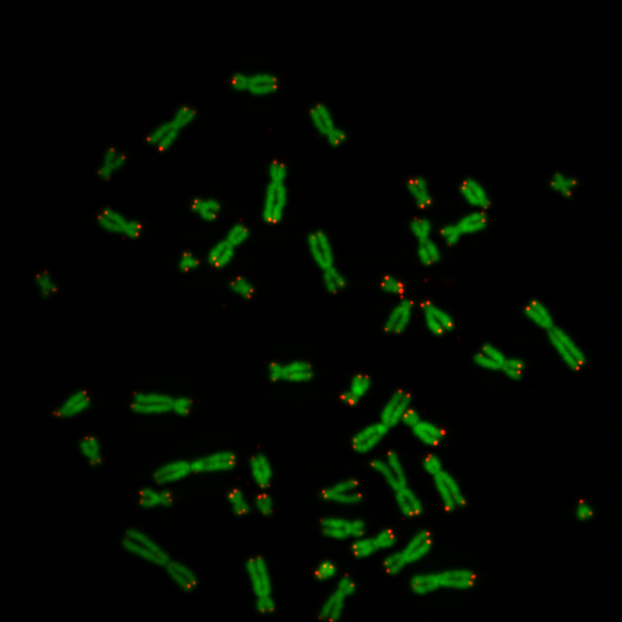
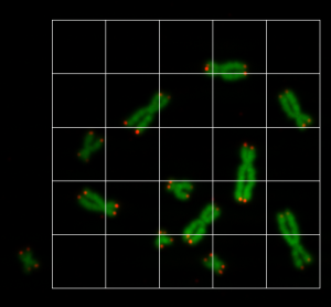
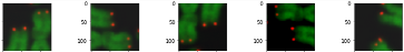
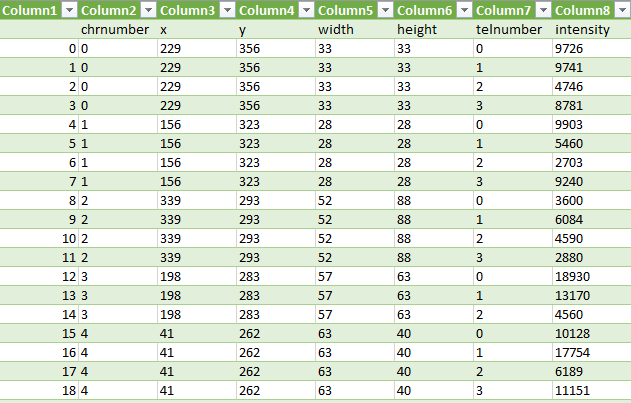
Previously we created with a tool around 3000 images from several complete chromosome images. We do not go much into detail about this tool. The tool works in a way that it loads in and shows a complete chromosome image with its 46 chromosomes and as an user we can select with the mouse a square on this image. The content of the square is then saved as a 128×128 chromosome image and as a 128×128 telomere image. Figure 1 shows an example of both images. We have created around 3000 chromosome and telomere images from different positions.
Each time we save the chromosome and telomere images, the application updates a csv file with the name of the chromosome (chrname) and the name of the telomere (telname) using the write function of the code below. It uses the library pandas to concat rows to the end of a csv file with the name f_name.
def write(chrname, telname, x, y):

    if isfile(f_name):

        df = pd.read_csv(f_name, index_col = 0)
        data = [{'chr': chrname, 'tel': telname, 'x': x, 'y':y}]
        latest = pd.DataFrame(data)
        df = pd.concat((df, latest), ignore_index = True, sort = False)
    else:
        data = [{'chr': chrname, 'tel': telname, 'x': x, 'y':y}]
        df = pd.DataFrame(data)

    df.to_csv(f_name)
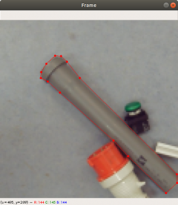
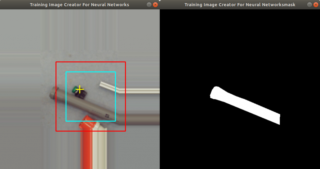
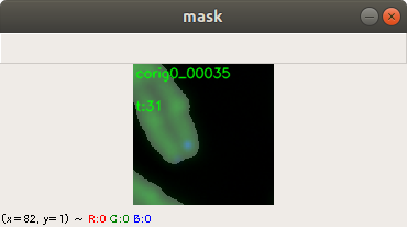
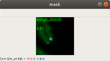
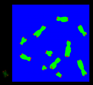
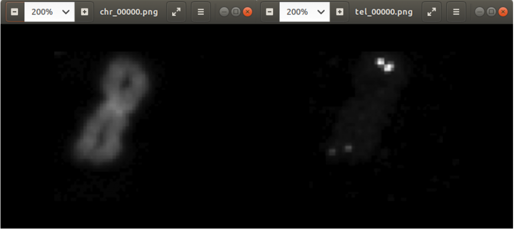
In the code above, you can see that a x and a y value is stored into the csv file, as well. This is the position of the centromere of the chromosome on the chromosome image. At this point of time, the position is not known yet. We need a tool, where we can click on each image to mark the centromere position. The code of the tool is shown below. There are two parts. The first part is the callback function click. It is called as soon as the user of the application presses a mouse button or moves the mouse. If the left mouse button is pressed, then the actual mouse position on the conc window is moved to the variable refPt. The second part of the tool loads in the a chromosome image from a directory chrdestpath and a telomere image from a directory teldestpath into a window named conc. The function makecolor (this function is described below) adds both images together to one image. The user can select with the mouse the centromere position and a cross appears on the clicking position, Figure 2. The application stores the position refPt by pressing the key “s” into the pandas data frame df. After this, the application loads in the next chromosome image from the directory chrdestpath and the next telomere image from the directory teldestpath.
refPt = (0,0)
mouseevent = False
def click(event,x,y,flags,param):
    global refPt
    global mouseevent
    if event == cv2.EVENT_LBUTTONDOWN:
        refPt = (x,y)
        mouseevent = True

cv2.namedWindow('conc')
cv2.setMouseCallback("conc", click)

theEnd = False
theNext = False

img_i=0
imgstart = 0
assert imgstart < imgcount

df = pd.read_csv(f_name, index_col = 0)

for index, row in df.iterrows():

    if img_i < imgstart:
        img_i = img_i + 1
        continue

    chrtest = cv2.imread("{}{}".format(chrdestpath,row["chr"]),1)
    teltest = cv2.imread("{}{}".format(teldestpath,row["tel"]),1)

    conc = makecolor(chrtest, teltest)
    concresized = np.zeros((conc.shape[0]*2, conc.shape[1]*2,3), np.uint8)
    concresized = cv2.resize(conc, (conc.shape[0]*2,conc.shape[1]*2), interpolation = cv2.INTER_AREA)

    refPt = (row["y"],row["x"])
    cv2.putText(concresized,row["chr"], (2,12), cv2.FONT_HERSHEY_SIMPLEX, 0.4, (0, 255, 0), 1, cv2.LINE_AA)

    while True:
        cv2.imshow('conc',concresized)
        key = cv2.waitKey(1)
        if mouseevent == True:
            print(refPt[0], refPt[1])
            concresized = cross(concresized, refPt[0], refPt[1], (255,255,255))
            mouseevent = False
        if key & 0xFF == ord("q") :
            theEnd = True
            break
        if key & 0xFF == ord("s") :
            df.loc[df["chr"] == row["chr"], "x"] = refPt[1]//2
            df.loc[df["chr"] == row["chr"], "y"] = refPt[0]//2
            theNext = True
            break
        if key & 0xFF == ord("n") :
            theNext = True
            break
    if theEnd == True:
        break
    if theNext == True:
        theNext = False

df.to_csv(f_name)
cv2.destroyAllWindows()
Figure 2 shows the cross added to the centromere position selected by the user. This procedure was done around 3000 times on chromosome and telomere images, so the output was a csv file with 3000 chromosome image names, telomere image names, and centromere positions.
Augmenting the Data
In general 3000 images are too few images to train a neuronal network, so we augmented the images to have more training data. This was done by mirrowing all chromosome images (and its centromere positions) on the horizontal axis and on the vertical axis. This increased the number of images to 12000. The code below shows the load_data function to load the training data or validation_data into arrays
def load_data(csvname, chrdatapathname, teldatapathname):
    X_train = []
    y_train = []

    assert isfile(csvname) == True
    df = pd.read_csv(csvname, index_col = 0)
    for index, row in df.iterrows():

        chrname = "{}{}".format(chrdatapathname,row["chr"])
        telname = "{}{}".format(teldatapathname,row["tel"])

        chrimg = cv2.imread(chrname,1)
        telimg = cv2.imread(telname,1)

        X_train.append(makecolor(chrimg, telimg))
        y_train.append((row['x'],row['y']))
    return X_train, y_train
In the code above you find a makecolor function. makecolor copies the grayscale images of the chromosome into the green layer of a new color image and the telomere image into the red layer of the same color image, see code of the function makecolor below.
def makecolor(chromo, telo):

    chromogray = cv2.cvtColor(chromo, cv2.COLOR_BGR2GRAY)
    telogray = cv2.cvtColor(telo, cv2.COLOR_BGR2GRAY)

    imgret = np.zeros((imgsize, imgsize,3), np.uint8)

    imgret[0:imgsize, 0:imgsize,1] = chromogray
    imgret[0:imgsize, 0:imgsize,0] = telogray

    return imgret
Below the function code mirrowdata to flip the images horizontally or vertically. It uses the parameter flip to control the flipping of the image and its centromere position.
 def mirrowdata(data, target, flip=0):
    xdata = []
    ytarget = []

    for picture in data:
        xdata.append(cv2.flip(picture, flip))

    for point in target:
        if flip == 0:
            ytarget.append((imgsize-point[0],point[1]))
        if flip == 1:
            ytarget.append((point[0],imgsize-point[1]))
        if flip == -1:
            ytarget.append((imgsize-point[0],imgsize-point[1]))

    return  xdata, ytarget
The following code loads in the training data into the array train_data and the array train_target. train_data contains color images of the chromosomes and telomeres and train_target contains the centromere positions. The mirrowdata function is applied twice on the data with different flip parameter settings. After this, the data is converted to numpy arrays. This needs to be done to be able to normalize the images with the mean function and the standard deviation function. This is done for 10000 images among the 12000 images for the training data. The same is done with the remaining 2000 images for the validation data.
train_data, train_target = load_data(csvtrainname, chrtrainpath, teltrainpath)
train_mirrow_data, train_mirrow_target = mirrowdata(train_data, train_target, 0)
train_data = train_data + train_mirrow_data
train_target = train_target + train_mirrow_target
train_mirrow_data, train_mirrow_target = mirrowdata(train_data, train_target, 1)
train_data = train_data + train_mirrow_data
train_target = train_target + train_mirrow_target

train_data = np.array(train_data, dtype=np.float32)
train_target = np.array(train_target, dtype=np.float32)

train_data -= train_data.mean()
train_data /= train_data.std()
Modeling and Training the Neuronal Network
Since we have images we want to feed into the neural network, we decided to use a neuronal network with convolution layers. We started with a Layer having 32 filters. As input for training data we need images with size imgsize, which is in our case 128. After each convolution layer we added the max pooling function with pool_size=(2,2) which reduces the size of the input data by half. The output is fed into the next layer. Altogether we have four convolution layers. The number of filters, we increase after each layer. After the fourth layer we flatten the network and feed this into the first dense layer. Then we feed the output into the second dense layer having only two neurons. The activation function is a linear function. This means, we will receive two float values, which is supposed to be the position of the centromere. As a loss function we decided to use the mean_absolute_percentage_error.
model = Sequential()
model.add(Conv2D(32, (3, 3), activation='relu', kernel_initializer='he_uniform', kernel_regularizer=l2(0.01), bias_regularizer=l2(0.01), padding='same', input_shape=(imgsize, imgsize, 3)))
model.add(MaxPooling2D((2, 2)))
model.add(Conv2D(32, (3, 3), activation='relu', kernel_initializer='he_uniform', kernel_regularizer=l2(0.01), bias_regularizer=l2(0.01), padding='same'))
model.add(MaxPooling2D((2, 2)))
model.add(Conv2D(64, (3, 3), activation='relu', kernel_initializer='he_uniform', kernel_regularizer=l2(0.01), bias_regularizer=l2(0.01), padding='same'))
model.add(MaxPooling2D((2, 2)))
model.add(Conv2D(128, (3, 3), activation='relu', kernel_initializer='he_uniform', kernel_regularizer=l2(0.01), bias_regularizer=l2(0.01), padding='same'))
model.add(MaxPooling2D((2, 2)))
model.add(Flatten())
model.add(Dense(128, activation='relu', kernel_initializer='he_uniform'))
model.add(Dropout(0.1))
model.add(Dense(2, activation='linear'))
opt = Adam(lr=1e-3, decay=1e-3 / 200)
model.compile(loss="mean_absolute_percentage_error", optimizer=opt, metrics=['accuracy'])
We start the training with the fit method. The input parameters are the list of colored and normalized chromosome images (train_data), the list of centromere positions (train_target), and the validation data (valid_data, valid_target). A callback function was defined to stop the training as soon as there is no progress seen. Also checkpoints are saved automatically, e.g. if there is progress during the training.
callbacks = [
    EarlyStopping(patience=10, verbose=1),
    ReduceLROnPlateau(factor=0.1, patience=3, min_lr=0.00001, verbose=1),
    ModelCheckpoint('modelregr.h5', verbose=1, save_best_only=True, save_weights_only=True)
]

model.fit(train_data, train_target, batch_size=20, nb_epoch=50, callbacks=callbacks, verbose=1, validation_data=(valid_data, valid_target) )
The training took around five minutes on a NVIDIA 2070 graphics card. The accuracy is 0.9462 and the validation accuracy is 0.9258. This shows a small overfitting. The loss function shows the same overfitting result.
Testing
We kept a few chromosome images and telomere images aside for testing and predicting. The images were stored in a test_data array and normalized before prediction. The prediction was done with the following code.
predictions_test = model.predict(test_data, batch_size=50, verbose=1)
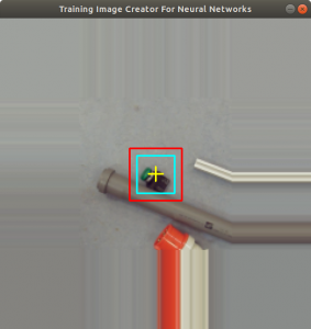
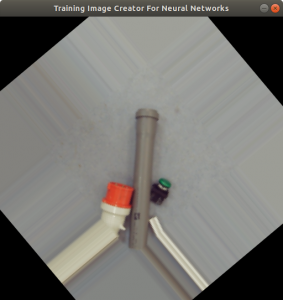
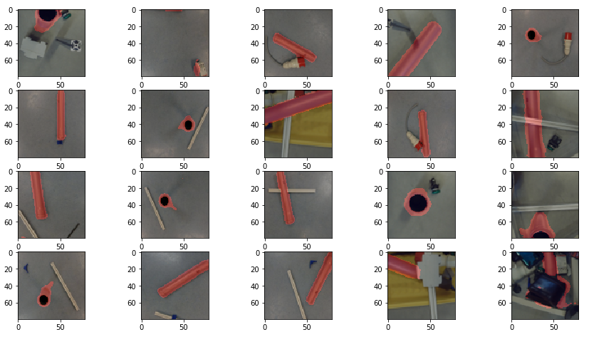
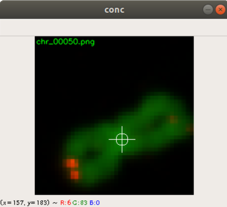
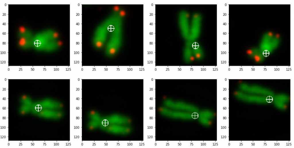
prediction_test contains now all predicted centromere positions. Figure 3 shows the positions added to the chromosome images. We can see that the position of the cross is pretty close to the centromere. However there are deviations.
For displaying the chromosomes as shown as in Figure 3 we use the following showpics function. Note in case you want to use this code, you have to be aware that the input images may not be normalized, otherwise you see see a black image.
def showpics(data, target, firstpics=0, lastpics=8):
    chrtail=[]
    pnttail=[]
    columns = 4
    print(data[0].shape)
    for i in range(firstpics, lastpics):
        chrtail.append(data[i])
        pnttail.append(target[i])
    rows = (lastpics-firstpics)//columns
    fig=figure(figsize=(16, 4*rows))
    for i in range(columns*rows):
        point = pnttail[i]
        fig.add_subplot(rows, columns, i+1)
        pic = np.zeros((chrtail[i].shape[0], chrtail[i].shape[1],3), np.uint8)
        pic[0:pic.shape[0], 0:pic.shape[1], 0] = chrtail[i][0:pic.shape[0], 0:pic.shape[1], 0]
        pic[0:pic.shape[0], 0:pic.shape[1], 1] = chrtail[i][0:pic.shape[0], 0:pic.shape[1], 1]
        pic[0:pic.shape[0], 0:pic.shape[1], 2] = chrtail[i][0:pic.shape[0], 0:pic.shape[1], 2]
        imshow(cross(pic, int(point[1]), int(point[0]), (255,255,255)))
Conclusion
The intention of this project was to show how to use linear regression as the last layer of the neuronal network. We wanted to get a position (coordinates) from an image.
Firstly we marked about 3000 centromere positions of chromosomes and telomere images with a tool we created. Then we augmented the data to increase the data to 12000 images. We augmented the data by horizontal and vertical flipping.
Secondly we trained a multilayer convolutional neural network with four convolutional layers and two dense layers. The last dense layer has two neurons. One for each coordinate.
The prediction result was fairly good, considering the little effort we used to optimize the model. On Figure 3 we still can see that the centromere position is not always hit on the right spot. We expect improvement after we will add more data and optimize the model.