At the school I work I am instructing a class called Design Cyber Physical Systems. The name of the class leaves many interpretations open about its content. However I leave this open intentionally. In the previous semesters, I let the students choose a topic, which has to do something with sensors, actors and micro-controllers. The students have to brainstorm a specific implementation idea, then they have to create a plan and execute the plan during the semester. This semester I changed the topic: This time the implementation idea has to contain a neural network and a camera system.
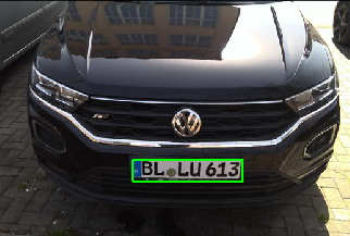
Three students who participated in this class decided to create a system which takes images from an access road having a gate towards a parking lot. As soon as a car approaches, the camera takes an image of the car with its license plate. The system has to determine the position of the license plate on the image and extract the license plate. Algorithms figure out the characters and numbers and compare them with the license plates stored in a database. If the license plate is identical to one of the license plates in the database, the gate is opened. Due to organizational problems with accessing a parking lot gate, we decided to use a simple signal light instead.
Data Preprocessing
The systems’s application needs first to find the license plate on the car’s image. This can be done in various ways, but we chose to use a neural network. We need to have many training images, which are images of cars from the front. We need to mark the license plates on each image to receive a new mask image needed for the neural network training.
There are already programs available, to download images, e.g. chromedriver. The program we used can be found here. You can control the search criteria with the options, and the program downloads automatically numerous images. The search criteria in our case was simply “license plate car”. Not every downloaded image served our purpose. We limited ourselves to German license plates, so we had to filter manually the useful images. Altogether we gathered around 760 training images and test images.
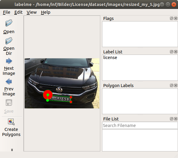
The next step was to label the areas of license plates of the downloaded images. We found a tool called labelme, which we had to install. Note that we managed to install only an older version of labelme on Ubuntu 18.04 (command: sudo pip3 install labelme==3.3.3). In Figure 1 you can see the tool labelme with an uploaded image. As a user you can click with the mouse around the license plate so a polygon is created. The points of the polygon can be saved into a json file. We have done this for all 760 images and 760 json files were created.
The next step was to create mask images from the json files. Each json file contained a number of points which was parsed by the function create_mask_from_image below. It opens the json file, retrieves the points, and uses skimage.draw‘s polygon method to create the mask image. Finally it stores the image to the mask_path directory.
from skimage.draw import polygon

def create_mask_from_image(path, json_file, img_width, img_height, file_number, output_dir):
    json_path = os.path.join(path, json_file)

    mask_name = "img_" + str(file_number) + ".png"
    mask_path = os.path.join(output_dir, "masks", mask_name)

    f = open(json_path)
    data = json.load(f)

    vertices = np.array([[point[1],point[0]] for point in data['shapes'][0]['points']])
    vertices = vertices.astype(int)

    img = np.zeros((img_height, img_width), 'uint8')

    rr, cc = polygon(vertices[:,0], vertices[:,1], img.shape)
    img[rr,cc] = 1

    imsave(mask_path, img)
This function was repeated for all available json files. So at this moment we had all training images and mask images stored in the paths dataset/images/ and dataset/masks/. Note that the names of the training images and the corresponding mask images need to be identical.
Training of the Neural Network
What we are facing is a segmentation problem. After we feed the application with an image of a car, we want to receive an image indicating where we find the license plate. A U-Net can be used to solve such a problem. In this blog this was already discussed on several posts, so see earlier posts. This time however we used the library keras_segmentation. The model is returned by the segnet method. We have chosen to use images with a height of 350 and a width of 525.
from keras_segmentation.models.segnet import segnet

model = segnet(n_classes=2, input_height=350, input_width=525)

path="/home/.../dataset/"

model.train(
    train_images =  path+"images/",
    train_annotations = path+"masks/",
    checkpoints_path = "/tmp/segnet", epochs=3
)

model.save("weights.h5")
The train method executes the training. On a NVIDIA 2070 graphic card it took about three minutes with three epochs with an accuracy of 99,4%. After training we saved the weights to a file called weights.h5.
Testing of the Neural Network
We have put a few images aside to test the trained model. The code below loads the model by using the method load_weights. A test image is read and shown with matplotlib’s imshow.
import matplotlib.pyplot as plt
import matplotlib.image as mpimg

model.load_weights("weights.h5")
img=mpimg.imread("/home/.../img_1.jpg")
imgplot = plt.imshow(img)
plt.show()
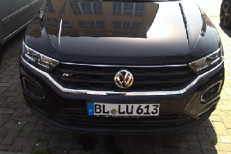
Figure 2 shows the test image from matplotlib. The license plate can be clearly seen at the lower/middle part of the image.
To predict the license plate area on the image, we need to feed the test image into the trained model. This can be done with the predict_segmentation method. This method writes the predicted image to out.png.
test_img = "/home/.../img_1.jpg"

out = model.predict_segmentation(
    inp=test_img,
    out_fname="dataset/tests/out.png",
)

plt.imshow(out)
The code above calls the matplotlib method imshow and in Figure 3 you can see the predicted mask image derived from the test image.

At the moment you cannot see how Figure 2 and Figure 3 overlap, so we wrote code to create an added image from the test image and the predicted mask image, see code below. Note that each pixel of the predicted mask image only has two values, zeros and ones. In order to add Figure 2 and Figure 3, we need to multiply the predicted mask image by 255. The OpenCV method addWeighted adds both images to a new image.
orig_img = cv2.imread(test_img)
out = out.astype('float32')
out = cv2.resize(out, (orig_img.shape[1], orig_img.shape[0]))
new_out = np.zeros((orig_img.shape[0], orig_img.shape[1], 3), dtype="uint8")
new_out[:,:,0] = out[:,:] * 255
orig_img = cv2.cvtColor(orig_img, cv2.COLOR_BGR2RGB)
plt.imshow(cv2.addWeighted(orig_img, 0.5, new_out, 0.5, 0.0))
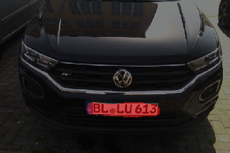
Matplotlib’s method imshow shows the added image, see Figure 4. You can see that both images align to each other very well. The license plate is highlighted with red color.
Position Detection of the License Plate
The next step is to find the position of the mask to receive a bounding box around the mask. We can use the OpenCV method findContours to receive the contour of the mask. The code below shows how we call findContours.
contours,_ = cv2.findContours(np.array(out, "uint8"), cv2.RETR_TREE, cv2.CHAIN_APPROX_SIMPLE)
plt.imshow(cv2.drawContours(orig_img, [contours[0]], -1, (255,0,0), 2))
Figure 5 shows the output image created by the OpenCV method drawContours.
The code below creates a bounding box from the contour around the license plate, which is assumed to be the first element of the output list contours. The OpenCV method boxPoints finds the rectangle with the corner points rect_corners having the minimum area around the contour. OpenCV’s drawContours draws the bounding box with matplotlib.
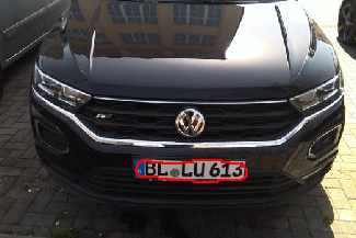
rect = cv2.minAreaRect(contours[0])
rect_corners = cv2.boxPoints(rect)
rect_corners = np.int0(rect_corners)

orig_img = mpimg.imread(test_img)
contour_img = cv2.drawContours(orig_img, [rect_corners], 0, (0,255,0),  2)
plt.imshow(contour_img)
In Figure 6 you can see how matplotlib draws the bounding box around the license plate. It is not generally true that the edges of the bounding box are in parallel to the edges of the test images. It is very possible, that the bounding rectangle is warped. This is something you cannot see in Figure 6.
Warping the License Plate Image
Before recognizing the letters of the license plate image, we should transform the bounding box to a real rectangular shape. The function order_points_clockwise of the code below sorts the points of rect_corners clockwise with the first point on the upper left corner. It returns the rearranged list to rect_corners_clockwise. The function warp_img extracts the license plate piece from the original test image and transform it to a real rectangle using the transformation methods getPerspectiveTransform and warpPerspective. The method warpPerspective receives the width and height of the extracted license plate with the function get_polygon_dimensions. Note again that the extracted license plate is not a real rectangle, but rather rhombus. The function get_polygon_dimensions uses Pythagoras for approximating the width and height of the rhombus. OpenCV’s method getPerspectiveTransform calcluates the transformation matrix and OpenCV’s method warpPerspective transforms the license plate image so it as a real rectangle shape.
def get_polygon_dimensions(points):
    from math import sqrt
    (tl, tr, br, bl) = points
    widthA = sqrt(((br[0] - bl[0]) ** 2) + ((br[1] - bl[1]) ** 2))
    widthB = sqrt(((tr[0] - tl[0]) ** 2) + ((tr[1] - tl[1]) ** 2))
    heightA = sqrt(((tr[0] - br[0]) ** 2) + ((tr[1] - br[1]) ** 2))
    heightB = sqrt(((tl[0] - bl[0]) ** 2) + ((tl[1] - bl[1]) ** 2))

    width = max(int(widthA), int(widthB))
    height = max(int(heightA), int(heightB))

    return (width, height)

def warp_img(img, points):
    width, height = get_polygon_dimensions(points)
    dst = np.array([
        [0, 0],
        [width - 1, 0],
        [width - 1, height - 1],
        [0, height - 1]], dtype = "float32")

    M = cv2.getPerspectiveTransform(points, dst)
    warped_img = cv2.warpPerspective(img, M, (width, height))

    return warped_img

def order_points_clockwise(pts):
    rect = np.zeros((4, 2), dtype="float32")

    s = pts.sum(axis=1)
    rect[0] = pts[np.argmin(s)]
    rect[2] = pts[np.argmax(s)]

    diff = np.diff(pts, axis=1)
    rect[1] = pts[np.argmin(diff)]
    rect[3] = pts[np.argmax(diff)]

    return rect

rect_corners_clockwise = order_points_clockwise(rect_corners)
orig_img = mpimg.imread(test_img)
warped_img = warp_img(orig_img, np.array(rect_corners_clockwise, "float32"))
plt.imshow(warped_img)

gray_img = cv2.cvtColor(warped_img, cv2.COLOR_RGB2GRAY)
_,prediction_img = cv2.threshold(gray_img, 50, 255, cv2.THRESH_BINARY)
plt.imshow(prediction_img)
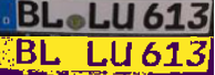
The upper part of Figure 7 you can see the image of the license plate piece from the original test image. The lower part of Figure 7 you can see the warped license plate image. It is converted to grayscale image combined with a threshold filter. Note that the warping in Figure 7 does not show much a difference. However the rectangle edges do not necessarily need to be in parallel with the test image edges, so transformation is really needed in some cases.
Character Recognition
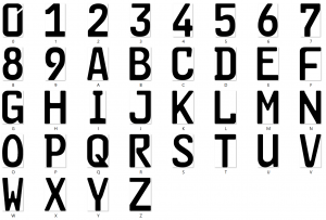
Figure 8 shows the set of reference characters for German license plates which are available as images for each character. In the code below the Figure, we set the directory with the reference character images to the variable feletterspath.
The main function from the code below is get_prediction which is called with a transformed and grayscaled license plate image as an input parameter.
First the function get_prediction finds the contours of the license plate image. The contours are forwarded to the _get_rectangles_around_letters function. It checks all contours’ height and width sizes with the function _check_dimensions. It simply figures out, if a contour has a similar height as the license plate image height and a similar width as one eighth of the license plate image width. If this is the case, there is a high probability that the contour is a character. The function _get_rectangles_around_letters sorts the contours from left to right using the sort function and moves the contours into the list rectangles. The contours in the list have now a high probability that they are characters.
feletterspath="/home/.../feletters/"

def get_prediction(img):

    img_dimensions = (660, 136)
    img = cv2.resize(img, (img_dimensions))

    contours,_ = cv2.findContours(img, cv2.RETR_CCOMP, cv2.CHAIN_APPROX_NONE)

    rectangles = _get_rectangles_around_letters(contours, img_dimensions)

    if len(rectangles) < 3:
        return

    letter_imgs = _get_letter_imgs(img, rectangles)
    letters = _get_letter_predictions(letter_imgs)
    letters = _add_space_characters(letters, rectangles)
    return letters


def _check_dimensions(img_dimensions, rectangle):

    img_width, img_height = img_dimensions
    (x,y,w,h) = rectangle
    letter_min_width, letter_max_width = img_width / 17, img_width / 8
    letter_min_height, letter_max_height = img_height / 2, img_height
    rectangle_within_dimensions = (w > letter_min_width and w < letter_max_width) \
        and (h > letter_min_height and h < letter_max_height)

    return rectangle_within_dimensions


def _get_rectangles_around_letters(contours, img_dimensions):

    rectangles = []

    for contour in contours:

        rectangle = cv2.boundingRect(contour)

        has_letter_dimensions = _check_dimensions(img_dimensions, rectangle)
        if has_letter_dimensions:
            rectangles.append(rectangle)

    rectangles.sort(key=lambda tup: tup[0])

    return rectangles
The function get_prediction from the code above is calling the function _get_letter_imgs from the code below to extract the character images from the input license plate image and returns a list. The function _get_letter_predictions iterates through this list and executes the function _match_fe_letter. The function _match_fe_letter is iterating through the set of license plate reference characters (shown in Figure 8) and applies the OpenCV matchTemplate method after the images are resized to the same shapes. OpenCV’s matchTemplate returns value indicating the similarity of the license plate character with the reference character. The license plate character with the highest similarity is chosen to be the matched character. Finally the function _get_letter_imgs returns a list of matched characters.
Figure 7 shows a space between the “BL” and “LU” and a space between “LU” and “613”. The function _add_space_characters adds a blank character between the matched characters, if the spaces of the character images exceed a certain threshold (20 in the code below).
def _get_letter_imgs(img, rectangles):

    letter_imgs = []

    for rect in rectangles:
        (x,y,w,h) = rect
        current_letter = img[y:y+h, x:x+w]
        letter_imgs.append(current_letter)

    return letter_imgs


def _get_letter_predictions(letter_imgs):

    letters = ""

    for letter_img in letter_imgs:
        prediction = _match_fe_letter(letter_img)
        letters += prediction

    return letters

def _add_space_characters(letters, rectangles):

    space_counter = 0

    for n,_ in enumerate(rectangles):
        (x1,_,w1,_) = rectangles[n]
        (x2,_,_,_) = rectangles[n+1]
        distance = x2-(x1+w1)

        if distance > 20:
            index = n + 1 + space_counter
            space_counter += 1
            letters = letters[:index] + ' ' + letters[index:]

        if n == len(rectangles)-2:
            break

    return letters


def _match_fe_letter(img):

    fe_letter_dir = feletterspath

    similarities = []

    for template_img in sorted(os.listdir(fe_letter_dir)):
        template = cv2.imread(os.path.join(fe_letter_dir, template_img), cv2.IMREAD_GRAYSCALE)
        img = cv2.resize(img, (template.shape[1], template.shape[0]))
        similarity = cv2.matchTemplate(img,template,cv2.TM_CCOEFF_NORMED)[0][0]
        similarities.append(similarity)

    letter_array = [os.path.splitext(letter)[0]
        for letter in sorted(os.listdir(fe_letter_dir))]

    letter = letter_array[similarities.index(max(similarities))]

    return letter
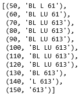
The function get_prediction is called several times with differently processed input images, see code below. The code calls OpenCV’s threshold with a range of thresholds and feeds the images into the method get_prediction. The result is appended to the results list.
results = []

for i in range(50,200,10):
    _,prediction_img = cv2.threshold(gray_img, i, 255, cv2.THRESH_BINARY)
    prediction = get_prediction(prediction_img)
    if prediction is not None:
        results.append((i,prediction))
Figure 9 shows the list of results from the license plate’s input image. You can see that the code correctly predicted the license plate six times. Here the majority of the same predictions can be used as a final predicted output.
Conclusion
In this blog I described a gate opening system designed by students from the class Design Cyber Physical Systems. The idea was, that a car approaches the gate, and a camera system takes images from the car including its license plate. We trained a neural network to receive a mask indicating the license plate’s position on the image. The application extracted the license plate with the mask from the image and applied character recognition supplied by OpenCV.
The application was actually distributed over two computers. One computer (raspberry pi) took images and controlled the output relay, the other computer calculated the mask image with a neural network. Actually we did not open a gate as described in the introduction. We connected a signal light to a relay which was controlled by the raspberry pi. The communication between both computers was realized by a REST interface.
The character recognition only worked well, if we fed the license plate image several times with different thresholds. A majority vote was taken to choose the recognized license plate number.
Acknowledgement
Thanks to Jonas Acker, Marc Bitzer and Thomas Schöller for participating at the class Design Cyber Physical Systems and providing the code which was the result of the project from this class.
Also special thanks to the University of Applied Science Albstadt-Sigmaringen offering a classroom and appliances to enable this research.